Satellite data shows CO2 does not control Earth's radiative balance or climate

Dr. Roy Spencer has an interesting post today analyzing several satellite datasets, which suggest "some portion of recent warming was simply due to a natural decrease in cloud cover."

Dr. Spencer also finds an independent method of determining Earth's radiative fluxes [fig 6 below], since "radiative fluxes are so important (e.g. being the basis for global warming theory) that any independent means of estimating them are worth looking into." "Be careful in interpreting the estimated radiative fluxes in Fig. 6 because they could have an offset. Since the anomalies I compute (by definition) sum to zero over the entire time series, that means the total time-integrated radiative energy flux also sums to zero. So, while the graph in Fig. 6 suggests energy loss by the global oceans over the last 5 years, it could be the whole curve needs to be shifted upward. There is no way to know."

I have overlaid the CO2 forcing from increased CO2 levels since 1987 as the red line in Dr. Spencer's Fig. 6 below, based upon the IPCC/Myhre formula for CO2 forcing due to the change in CO2 levels of 349.16 ppm in 1987 to 400 ppm today,

5.35*ln(400/349.16)=0.73 W/m2

which clearly illustrates a disconnect between CO2 levels and net radiative flux, and demonstrates CO2 radiative forcing is not the so-called climate "control knob."

However, all IPCC models are based upon the IPCC/Myhre formula for CO2 radiative forcing, and despite the complexity of the models, the global warming predictions essentially follow this simple formula 1:1:

You don't even need a climate model to show what climate models predict - projections are based upon a single independent variable - CO2 

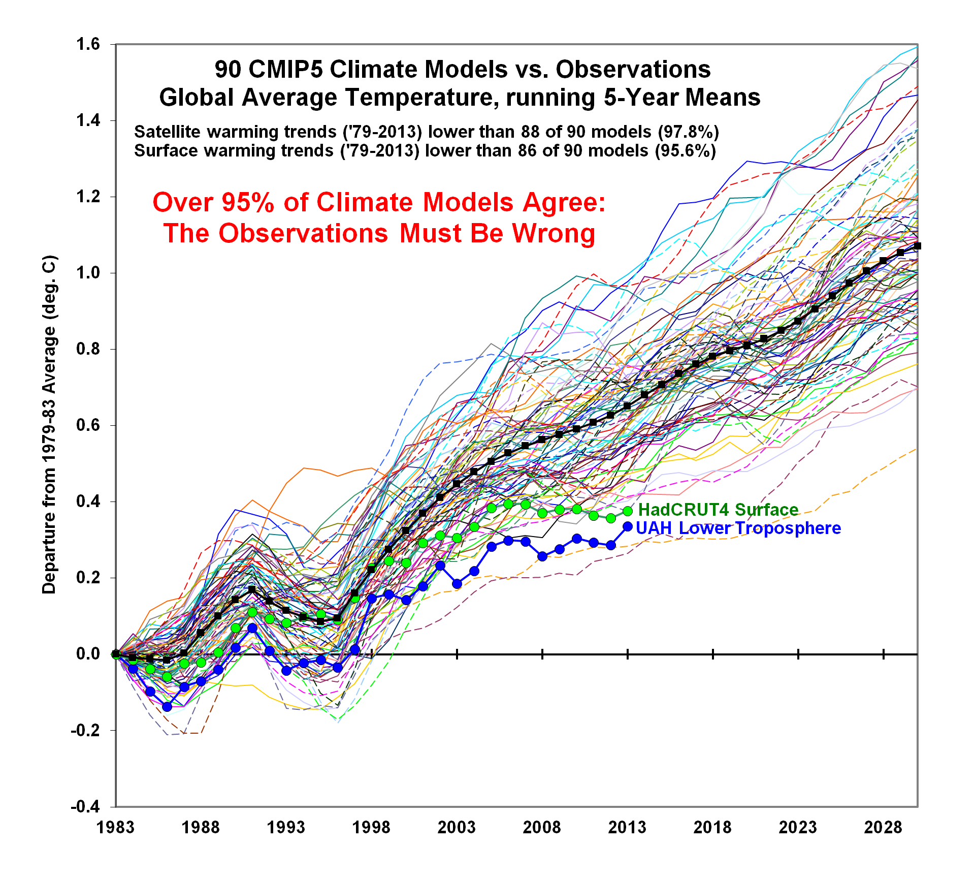
Thus explaining why the models have been falsified at confidence levels exceeding 98%.

SSM/I Global Ocean Product Update: Increasing clouds with a chance of cooling

by Roy W. Spencer, Ph. D.

My research field of satellite passive microwave remote sensing took off like a rocket (pun intended) when the first Special Sensor Microwave/Imager (SSM/I, built by Hughes Aircraft) was launched in mid-1987 on the DoD series of weather satellites (DMSP).

We SO anticipated that first instrument…good calibration, and high frequency channels to estimate precipitation over land. The previous NASA instruments (ESMR-5, -6, and SMMR) were a good start, but had limited channel selection and less than optimal calibration strategies.

The SSM/I instrument series was later redesigned to incorporate the temperature sounding channels (SSMIS, built by Aerojet). (By the way, we don’t use these in our UAH global temperature monitoring work, since we receive very little money to produce the UAH datasets and incorporating an entirely new series of instruments would be a major effort).

But the real benefit of the SSM/I series of satellite sensors was the production of the “ocean suite” of products: integrated water vapor, surface wind speed, integrated cloud water, and rain rate. These continue to be produced by several investigators, and I use those produced by Remote Sensing Systems (RSS).

To help interpret the SSM/I measurements, let’s start with the HadSST3 sea surface temperatures (SSTs) measured since July, 1987, which is when SSM/I data first became available. (All of the following time series are monthly global anomalies since July, 1987; some have trailing 6-month averages plotted as well). It shows the well-known warming up until the 1997/98 El Nino, then roughly level temperatures since then.

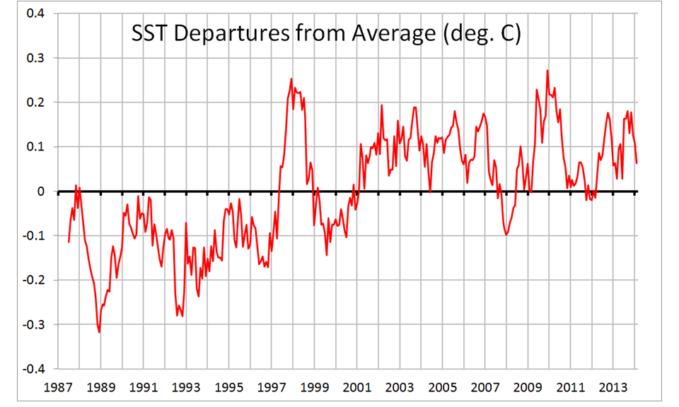Fig. 1. Monthly global oceanic HadSST3 anomalies from July 1987 thru Feb. 2014.

The first SSM/I field to address is total vertically-integrated water vapor, which closely follows the SST variations:

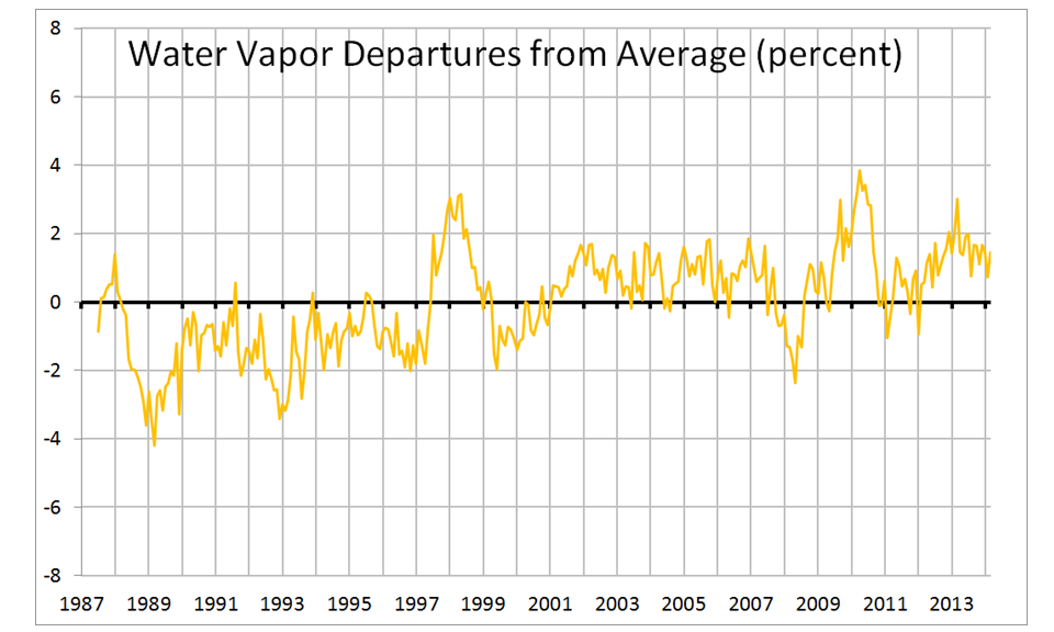Fig. 2. Monthly global oceanic anomalies in SSM/I total integrated water vapor.

The water vapor variations lag the SST variations by an average of one month. A regression relationship reveals an average 10.2% increase in vapor per deg. C increase in SST. This is larger than the theoretically-expected value of 6.5% to 7% increase, a discrepancy which can be interpreted in different ways (more evaporative cooling of the ocean stabilizing the climate, or more water vapor feedback destabilizing the climate — take your pick).

Next, let’s examine the surface wind speed variations from SSM/I. These have been compared to literally millions of buoy wind measurements, and are quite accurate. In fact, I would wager these are by far the best estimate of changes in global ocean wind speed we have:

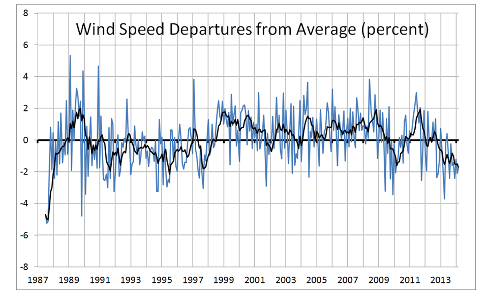Fig. 3. Monthly global oceanic anomalies in surface wind speed from SSM/I.

We see there was a slight (1-2%) increase in ocean wind speed from before the 1997/98 El Nino to after, which at least qualitatively might be supportive of Trenberth’s claim of increase ocean heat storage and surface cooling temporarily cancelling out anthropogenic global warming. I have not looked into whether a 1-2% change in wind speed could have such an effect, so feel free to comment on this. Note also that the last year or so hints at a reversal of this increase back to pre-1998 wind speeds. If wind speeds remain at the lower level, it will be interesting to see if surface warming resumes. I’m making no predictions on this.

The SSM/I rain rate variations are always quite noisy. Warm conditions tend to show more rainfall, but the strong 1997/98 El Nino curiously shows little effect, and there is a hint of increasing ocean rainfall in recent years:

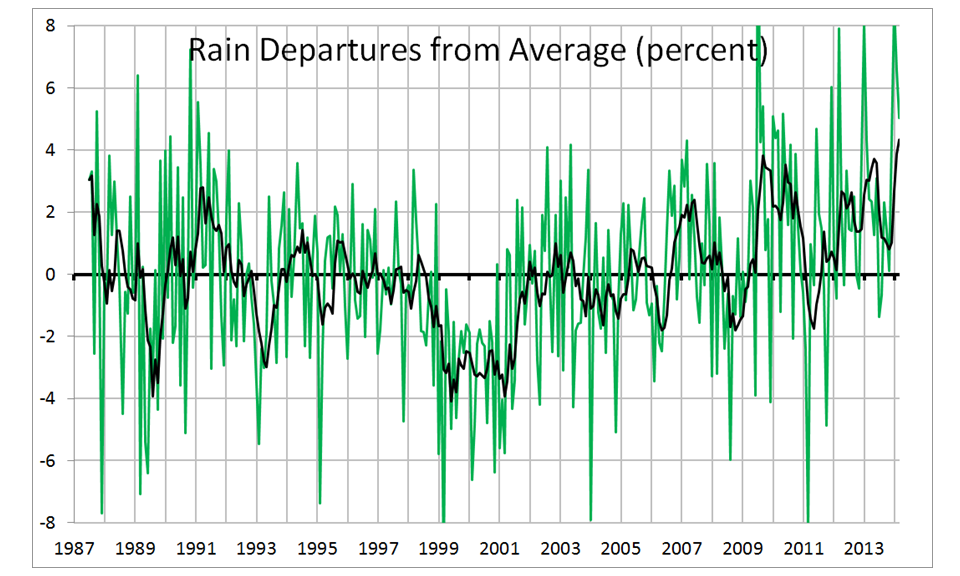Fig. 4. Monthly global oceanic anomalies in rainfall from SSM/I.

Finally, let’s look at what I think is the most interesting SSM/I variable from a climate change standpoint, total integrated cloud liquid water (CLW):

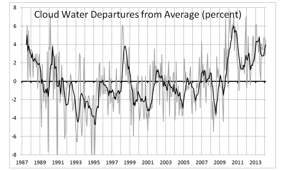Fig. 5. Monthly global oceanic anomalies in integrated cloud water from SSM/I.

The variations in cloud water show some interesting low-frequency behavior. I have previously discussed the fact that these cloud water variations are correlated with CERES-measured net radiative flux, and so provide a proxy measurement for the net radiative imbalance over the ocean which suggest some portion of recent warming was simple due to a natural decrease in cloud cover.

The updated regression relationship I get is 0.24 W/m2 loss in Net (solar plus IR) radiative energy for each percent increase in SSM/I cloud water, a scale factor we can then apply to the cloud water graph to get a Net radiative flux graph:

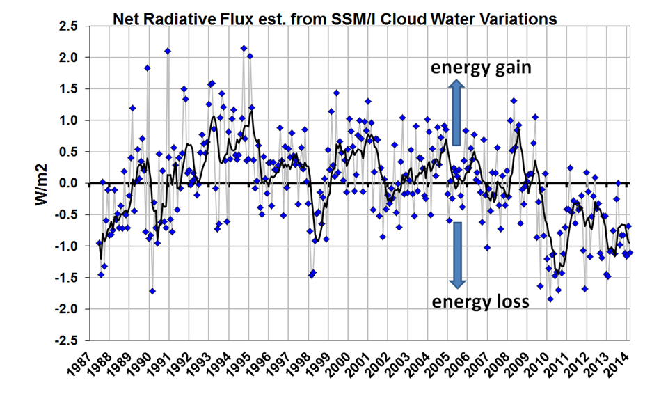Fig. 6. Monthly global oceanic anomalies in Net radiative flux estimated from SSM/I cloud water variations, using a CERES-based scale factor of 0.24 W/m2 per percent cloud water change.

Why use an SSM/I estimate of CERES Net radiative flux, instead of CERES directly? Mostly because CERES is available only since 2000, whereas SSM/I is available since 1987. But also, the CERES measurements are very difficult, with the reflected solar flux (which dominates the CERES-SSM/I relationship) having a strong angular dependence. The SSM/I measurements are instead thermally-based (microwave emission) and have no such angular dependence. Finally, radiative fluxes are so important (e.g. being the basis for global warming theory) that any independent means of estimating them are worth looking into.

Be careful in interpreting the estimated radiative fluxes in Fig. 6 because they could have an offset. Since the anomalies I compute (by definition) sum to zero over the entire time series, that means the total time-integrated radiative energy flux also sums to zero. So, while the graph in Fig. 6 suggests energy loss by the global oceans over the last 5 years, it could be the whole curve needs to be shifted upward. There is no way to know. The CERES fluxes have already been adjusted to match the increase in oceanic heat content, which was a logical thing for the CERES Team to do since the absolute accuracy of CERES is ~10 W/m2, whereas the increase in ocean heat content in recent years (IF you believe the warming estimates) correspond to only a few tenths of a W/m2 imbalance. The main value in the graph is to identify possible changes over time.

Others might see some relationships in the above plots that I haven’t noticed; I’ve made the Excel spreadsheet available for those who want to play with the data.

New paper finds sea level trends are biased by natural ocean oscillations

A new paper published in Geophysical Research Letters finds that much of the observed variation in Pacific Ocean sea levels is explained by natural ocean oscillations such as the Pacific Decadal Oscillation [PDO] and El Nino Southern Oscillation [ENSO]. The authors caution that sea level trends over the short period observed by satellites [less than 20 years] can be erroneously biased by this natural variability.

Top graph shows rapid sea level changes in the Western Pacific and little to no sea level change in the Eastern Pacific since 1993 are largely due to natural variability from ocean oscillations [ENSO and PDO]

GEOPHYSICAL RESEARCH LETTERS, VOL. 39, L21701, 8 PP., 2012

doi:10.1029/2012GL053240

Sea level trends, interannual and decadal variability in the Pacific Ocean

Key Points

• Sea level linear trend over short period is complicated by climate variability
• We separate interannual and decadal sea level variability from trend in Pacific
• Decadal sea level [natural] variability can be erroneously aliased into sea level trend

Xuebin Zhang

Centre for Australian Weather and Climate Research, a Partnership between CSIRO and the Bureau of Australia Meteorology, Melbourne, Victoria, Australia

CSIRO Wealth from Oceans Flagship, Hobart, Tasmania, Australia

CSIRO Marine and Atmospheric Research, Hobart, Tasmania, Australia

John A. Church

Centre for Australian Weather and Climate Research, a Partnership between CSIRO and the Bureau of Australia Meteorology, Melbourne, Victoria, Australia

CSIRO Wealth from Oceans Flagship, Hobart, Tasmania, Australia

CSIRO Marine and Atmospheric Research, Hobart, Tasmania, Australia

Linear trend analysis is commonly applied to quantify sea level change, often over short periods because of limited data availability. However, the linear trend computed over short periods is complicated by large-scale climate variability which can affect regional sea level on interannual to inter-decadal time scales. As a result, the meaning of a local linear sea level trend over the short altimeter era (since 1993; less than 20 years) is unclear, and it is not straightforward to distinguish the regional sea level changes associated with climate change from those associated with natural climate variability. In this study, we use continuous near-global altimeter measurements since 1993 to attempt to separate interannual and decadal sea level variability in the Pacific from the sea level trend. We conclude that the rapid rates of sea level rise in the western tropical Pacific found from a single variable linear regression analysis are partially due to basin-scale decadal [natural] climate variability. The negligible sea level rise, or even falling sea level, in the eastern tropical Pacific and US west coast is a result of the combination of decreasing of sea level associated with decadal [natural] climate variability and a positive sea level trend. The single variable linear regression analysis only accounts for slightly more than 20% of the observed variance, whereas a multiple variable linear regression including filtered indices of the El Nino-Southern Oscillation and the Pacific Decadal Oscillation accounts for almost 60% of the observed variance.

New paper shows California/Southwest US droughts are at some of the lowest levels of past 3000 years

A paper published today in Quaternary Science Reviews is the first to reconstruct droughts in California and the Southwest US for the past 3000 years and clearly demonstrates drought conditions were far more severe and persistent in the distant past than during recent history. In fact, the paper demonstrates drought at the end of the record is at some of the lowest levels of the past 3,000 years and far more extreme epic droughts in the US Southwest/California have persisted for periods of 300-500 years at least three times over the past 3 millennia. 

The authors find wet conditions are associated with more frequent El Ninos, and droughts with periods having fewer El Ninos. Although some climate scientists such as Kevin Trenberth have claimed AGW will cause more frequent El Ninos [and thus less drought], the El Nino reconstruction in this paper shows the frequency of El Ninos in the past 3000 years has been persistently much higher and much lower than the present for periods lasting several hundred years each.

Bottom line is that this paper demolishes claims that current California drought conditions are relatively "extreme" or linked to man-made CO2, as well as claims that man-made CO2 controls the frequency of natural El Ninos. 

Horizontal axis is calendar years before the present [BP] over the past 3000 years [most recent history at left side of graph], vertical axis is a proxy of wetness with higher values indicating more precipitation and less drought. Green line shows recent drought area (%) is at some of the lowest levels of past 1,100 years. 

Horizontal axis is calendar years before the present [BP] over the past 3000 years, bottom graph shows a proxy of wetness with higher values indicating more precipitation and less drought, most recent values at some of the highest wetness/lowest drought levels of the past 3000 years. Middle graph shows frequency of El Ninos in recent past is about in the middle of the range of extremes over the past 3000 years. 

Tropical Pacific forcing of Late-Holocene hydrologic variability in the coastal southwest United States

• Matthew E. Kirby^a, , , 
• Sarah J. Feakins^b, , , 
• Christine A. Hiner^a, 
• Joanna Fantozzi^a, 
• Susan R.H. Zimmerman^c, 
• Theodore Dingemans^d, 
• Scott A. Mensing

Highlights

•

3000 year decadal resolution record from Zaca Lake, CA.

•

Winter season moisture source and run-off reconstruction.

•

Pluvial or drought conditions associated with variable moisture sources.

•

Record extends knowledge of drought beyond tree ring reconstructions.

•

Evidence for persistent coupling between El Niño and run-off over 3000 years.

---

Abstract

Change in water availability is of great concern in the coastal southwest United States (_CSWUS). Reconstructing the history of water pre–1800 AD requires the use of proxy data. Lakes provide long-lived, high-resolution terrestrial archives of past hydrologic change, and their sediments contain a variety of proxies. This study presents geochemical and sedimentological data from Zaca Lake, CA (Santa Barbara County) used to reconstruct a 3000 year history of winter season moisture source (δD_wax) and catchment run-off (125–2000 μm sand) at decadal resolution. Here we show that winter season moisture source and run-off are highly variable over the past 3000 years; superimposed are regime shifts between wetter or drier conditions that persist on average over multiple centuries. Moisture source and run-off do not consistently covary indicating multiple atmospheric circulation modes where wetter/drier conditions prevail. Grain-size analysis reveals two intervals of multi-century drought with less run-off that pre-date the “epic droughts” as identified by Cook et al. (2004). A well-defined wet period with more run-off is identified during the Little Ice Age. Notably, the grain size data show strong coherence with western North American percent drought area indices for the past 1000 years. As a result, our data extend the history of drought and pluvials back to 3000 calendar years BP in the _CSWUS [coastal southwest United States]. Comparison to tropical Pacific proxies confirms the long-term relationship between El Niño and enhanced run-off in the _CSWUS [coastal southwest United States]. Our results demonstrate the long-term importance of the tropical Pacific to the _CSWUS [coastal southwest United States] winter season hydroclimate.

New paper: Dubious claims about California ocean habitat derived from tree-rings

Headlines today proclaim "Nearly 600 Years of Tree Rings Show Altered Ocean Habitat" due to an alleged weakening of the California Pacific Ocean coastal upwelling current, based on a paper published in Science.

Examination of the assumptions and data from the paper, however, illustrates how alarming claims in the press can be manufactured from very little scientific evidence. 

Questionable claims include:

1. Assuming the California Pacific Ocean upwelling current strength and variability are closely correlated to tree-rings, which is the proxy used, rather than ocean sediments or an actual ocean proxy.

2. Claiming [in article below the abstract] that the California Pacific Ocean upwelling current strength has weakened in the latter half of the 20th century, while the data below shows no such trend in the tree-ring proxy.

3. Claiming that the California Pacific Ocean upwelling current strength has become more variable because the moisy tree-ring proxy record has a few extra one-year-long dips as indicated by red arrows at the top of the graph below. 

a) these could simply be due to random variation in the very noisy record

b) tree-rings can be related to many factors other than precipitation and temperature, including cloud cover/cosmic rays, solar activity, CO2 plant food levels, ocean & atmospheric oscillations, etc., thus the alleged "increased variability" may not be related to upwelling current changes. 

c) the authors find these dips correlated to El Ninos, which were not exceptionally strong or variable during the latter 20th century, and have become less frequent and weaker since the beginning of the 21st century.

Thus, the paper is based upon multiple questionable assumptions that do not warrant the claims of an alarming trend in marine productivity due to an alleged weakening of coastal upwelling along the California coast.

Tree-ring data from the paper

Editor's Summary:

Rings of ocean upwelling

Coastal upwelling along the coast of California has become more variable than during nearly any period in the past 600 years. Black et al. used a 576-year tree ring record to construct a record of wintertime climate along the California coast. Because wintertime climate depends heavily on coastal upwelling, they were able to determine that upwelling variability has increased more over the past 60 years than for all but two intervals during that time. The apparent causes of the recent trend appear to be unique, resulting in reduced marine productivity and negative impacts on fish, seabirds, and mammals.


Science 19 September 2014:
Vol. 345 no. 6203 pp. 1498-1502
DOI: 10.1126/science.1253209

Six centuries of variability and extremes in a coupled marine-terrestrial ecosystem

Bryan A. Black, et al

Reported trends in the mean and variability of coastal upwelling in eastern boundary currents have raised concerns about the future of these highly productive and biodiverse marine ecosystems. However, the instrumental records on which these estimates are based are insufficiently long to determine whether such trends exceed preindustrial limits. In the California Current, a 576-year reconstruction of climate variables associated with winter upwelling indicates that variability increased over the latter 20th century to levels equaled only twice during the past 600 years. This modern trend in variance may be unique, because it appears to be driven by an unprecedented succession of extreme, downwelling-favorable, winter climate conditions that profoundly reduce productivity for marine predators of commercial and conservation interest.

Nearly 600 Years of Tree Rings Show Altered Ocean Habitat

By Kelly Dickerson, Staff Writer | September 18, 2014 02:35pm ET




Ocean currents that deliver important nutrients to shallow, coastal waters have become weaker and more variable over the last half-century, which could affect fish and other marine animals that nourish themselves in these nutrient-rich waters, according to a new study.

Data records spanning almost 600 years have shown that the strength of coastal upwelling off the west coast of North America has become more variable since 1950. Researchers pieced together this long-term look at ocean trends from an unlikely source: tree rings.

Coastal upwelling happens when winter winds lift deep, nutrient-rich waters up to the shallow layers of the sea. These nutrients fuel phytoplankton growth in the sunlit surface waters. Since 1950, California has experienced more winters with weak coastal upwelling than in the last five centuries. Researchers found that years with weak upwelling were associated with slower growth in fish populations and lower reproduction rates for seabirds, the researchers said.

But the weather pattern that causes the coastal upwelling also blocks storms from coming ashore. This causes drought and stunts the growth of trees. Blue oak trees along the California coast are particularly sensitive to winter precipitation, Bryan Black, assistant professor of marine science at the University of Texas at Austin, told Live Science.

Trees grow a new ring every year. By looking at a cross-section cut through the bark of a tree, scientists can count up the rings and determine a tree's age. Differences in the ring sizes reveal good seasons and bad seasons, with a thick ring signaling that the tree had a good growing season. The researchers found an inverse relationship between tree growth and the well-being of the marine ecosystem, Black explained.

"The winters we see robust growth in the trees, we see poor growth in the marine ecosystem," Black said.
Coastal upwelling happens during the winter when a strong, high-pressure weather system develops along the west coast of the continent. The system spins clockwise and brings in winds from the north. That spin combines with the rotation of the Earth to move the waters off shore and stir up clouds of nutrients. Phytoplankton at the surface rely on this seasonal influx of nutrients. These organisms are the backbone of the marine ecosystem and support huge populations of fish and seabirds.

Some variation in coastal upwelling from year to year is normal, but most direct data records don't go back more than 70 years. This makes it difficult for marine scientists to spot any long-term trends. By studying tree-ring patterns, however, researchers can piece together a much longer record of how coastal upwelling has changed.
To determine how upwelling influenced marine life, the researchers used data on yearly fish population growth since the 1940s, along with data on seabird egg laying and the survival of baby seabirds since the 1970s. By comparing the tree-ring data to the fish and seabird statistics, the researchers found that years with weak upwelling and lots of tree growth correlated with years when fish and seabird populations suffered.

Based on tree ring measurements taken by David Stahle, a tree ring expert and professor of geoscience at the University of Arkansas in Fayetteville, the team found that four out of the 10 weakest upwelling years in the past 600 years occurred after 1950. Seven out of 10 weakest years have happened since 1850 [the end of the Little Ice Age].

While the data show there are years in which bird and fish populations don't fare well, "it's not necessarily indicative of a long-term decline," Black said, since the bird and fish populations usually bounce back within a couple years after a bad season.
Black said it's unclear if climate change is causing the recent high variation in coastal upwelling.

"California climate can be very extreme," Black said. "The 20th century is particularly variable in the context of the last few centuries, but it's not necessarily unique to history."

The upwelling does appear to be linked to the weather pattern El Niño, and climate records have shown El Niño to be unusually variable over the past century. [not according to many other papers - El Nino's were much more intense & variable in the past]. Black said the area has certainly entered a highly variable time, but even a 600-year data record doesn't come close to capturing the whole picture. The recent variation could be part of a larger cycle that scientists can look back far enough to see.

The researchers hope to use [falsified] climate models to predict future variability in coastal upwelling. Details of the study were published online today (Sept. 18) in the journal Science.

New paper finds El Ninos were much more extreme in the past

A new paper published in Quaternary Science Reviews reconstructs the climate of tropical Western Australia over the past 9,000 years and finds the intensity of the Indonesian–Australian summer monsoon (IASM), which is driven by ENSO/El Nino activity, has declined over the past 5,000 years since the Holocene Climate Optimum. The paper adds to many other peer-reviewed publications demonstrating that, contrary to claims of climate alarmists, present-day climate is less variable and less extreme than during most of the Holocene [the past ~11,000 years].

Vertical axis shows d18O, a proxy of temperature and precipitation.
Horizontal axis is thousands of years before the present.

Frequency of El Ninos per 100 years shown in red in top graph. Charcoal abundance, a proxy of fire activity, is shown in orange in second graph and also indicates a decline over the past 4,000 years. Horizontal axis is thousands of years before the present.

A Stalagmite record of Holocene Indonesian–Australian summer monsoon variability from the Australian tropics

• Rhawn F. Denniston^a, , , 
• Karl-Heinz Wyrwoll^b, 
• Victor J. Polyak^c, 
• Josephine R. Brown^d, 
• Yemane Asmerom^c, 
• Alan D. Wanamaker Jr.^e, 
• Zachary LaPointe^c, 
• Rebecca Ellerbroek^a, 
• Michael Barthelmes^a,
• Daniel Cleary^a, 
• John Cugley^f, 
• David Woods^g, 
• William F. Humphreys^b, h, i

• ^a Department of Geology, Cornell College, Mount Vernon, IA, USA
• ^b University of Western Australia, Perth, Western Australia, Australia
• ^c Department of Earth and Planetary Sciences, University of New Mexico, Albuquerque, NM, USA
• ^d Centre for Australian Weather and Climate Research, Melbourne, Australia
• ^e Department of Geological and Atmospheric Sciences, Iowa State University, Ames, IA, USA
• ^f Kimberley Toad Busters, Kununurra, Western Australia, Australia
• ^g Department of Environment and Conservation, Broome, Western Australia, Australia
• ^h Western Australian Museum, Welshpool DC, Western Australia, Australia
• ⁱ University of Adelaide, Adelaide, South Australia, Australia

Highlights

•

Holocene IASM reconstructed for tropical Western Australia.

•

Phasing of monsoon strength similar to Borneo but opposite to Flores.

•

ENSO, not ITCZ, best explains monsoon variability.

•

Weak Late Holocene monsoon tied to peak El Niño activity.

---

Abstract

Oxygen isotopic data from a suite of calcite and aragonite stalagmites from cave KNI-51, located in the eastern Kimberley region of tropical Western Australia, represent the first absolute-dated, high-resolution speleothem record of the Holocene Indonesian–Australian summer monsoon (IASM) from the Australian tropics. Stalagmite oxygen isotopic values track monsoon intensity via amount effects in precipitation and reveal a dynamic Holocene IASM which strengthened in the early Holocene, decreased in strength by 4 ka, with a further decrease from ∼2 to 1 ka, before strengthening again at 1 ka to years to levels similar to those between 4 and 2 ka. The relationships between the KNI-51 IASM reconstruction and those from published speleothem time series from Flores and Borneo, in combination with other data sets, appear largely inconsistent with changes in the position and/or organization of the Intertropical Convergence Zone (ITCZ). Instead, we argue that the El Niño/Southern Oscillation (ENSO) may have played a dominant role in driving IASM variability since at least the middle Holocene. Given the muted modern monsoon rainfall responses to most El Niño events in the Kimberley, an impact of ENSO on regional monsoon precipitation over northwestern Australia would suggest non-stationarity in the long-term relationship between ENSO forcing and IASM rainfall, possibly due to changes in the mean state of the tropical Pacific over the Holocene.

Settled science update: 'Greenhouse gases' don't cause sea level rise

A paper published this week in The Journal of Climate finds the "settled" belief that warming due to 'radiative forcing' from 'greenhouse gases' is causing the seas to rise is not supported by observational data. The authors "find a relationship between sea level and temperature and find that temperature causally depends on the sea level, which can be understood as a consequence of the large heat capacity of the ocean." In other words, increase in surface temperature is caused by sea level rise rather than the "consensus" belief that temperature causes sea level rise. Furthermore, the authors attempt to find evidence that 'radiative forcing' from 'greenhouse gases' caused sea level rise in the latter 20th century, "but unexpectedly find that the sea level does not depend on the forcing." This is of no surprise to some skeptics who understand downwelling infrared from 'greenhouse gases' is incapable of heating the ocean due to a penetration depth of only a few microns.

Hansen's corrupted temperature anomalies in top graph, corrupted sea level in second graph, total 'radiative forcing' anomalies from greenhouse gases in third graph. Also note graphs stop in ~1998 during a record El Nino and that temperature and sea levels have declined since in some datasets.

Journal of Climate 2012 ; e-View

doi: http://dx.doi.org/10.1175/JCLI-D-11-00598.1

Statistical analysis of global surface temperature and sea level using cointegration methods

Torben Schmith¹

Danish Meteorological Institute, Copenhagen, Denmark

Søren Johansen

University of Copenhagen, Copenhagen, Denmark

Peter Thejll

Danish Meteorological Institute, Copenhagen, Denmark

Abstract

Global sea level rise is widely understood as a consequence of thermal expansion and melting of glaciers and land-based ice caps. Due to the lack of representation of ice-sheet dynamics in present-day physically-based climate models, semi-empirical models have been applied as an alternative for projecting of future sea levels. There are in this, however, potential pitfalls due to the trending nature of the time series. We apply a statistical method called cointegration analysis to observed global sea level and land-ocean surface temperature, capable of handling such peculiarities. We find a relationship between sea level and temperature and find that temperature causally depends on the sea level, which can be understood as a consequence of the large heat capacity of the ocean. We further find that the warming episode in the 1940s is exceptional in the sense that sea level and warming deviates from the expected relationship. This suggests that this warming episode is mainly due to internal dynamics of the ocean rather than external radiative forcing. On the other hand, the present warming follows the expected relationship, suggesting that it is mainly due to radiative forcing. In a second step, we use the total radiative forcing as an explanatory variable, but unexpectedly find that the sea level does not depend on the forcing. We hypothesize that this is due to a long adjustment time scale of the ocean and show that the number of years of data needed to build statistical models that have the relationship expected from physics exceeds what is currently available by a factor of almost ten.


Full paper here