Christopher Monckton has replied to the critique posted at Climate, etc. regarding the Monckton, Soon, Legates, and Briggs paper “Why models run hot, results from an irreducibly simple climate model,” and makes a number of good points highlighted below.
By Christopher Monckton of Brenchley
I am most grateful to Rud Istvan for his thoughtful commentary on our paper Why
models run hot: results from an irreducibly simple climate model, which appeared
in Vol. 60 no. 1 (January 2015) of the Science Bulletin of the Chinese Academy of
Sciences and the National Natural Science Foundation of China.
Dr Istvan kindly points out that the Science Bulletin is the Orient’s equivalent of
Science or Nature. Peer review, contrary to the sneering comments of the profiteers
of doom, was professional and thorough, requiring us to work quite hard to meet the
challenges – some of them from out of left field – that our three diligent and
commendably persistent reviewers presented.
He also dismisses – rightly – the hasty comments of Dr Trenberth, who did himself
no favors and us no harm by saying our model is very simple and the climate isn’t.
Well, every model is a simplification, and every simplification is an analogy, and
every analogy breaks down at some point.
Interestingly, though, because the climate behaves as a chaotic object a simple model
is not inherently less likely to be able to reach a respectable projection of climate
sensitivity than a far more complex model.
As Edward N. Lorenz pointed out in the elegant landmark paper Deterministic nonperiodic
flow that founded chaos theory in the Journal of the Atmospheric Sciences
in 1963, (though Lorenz did not use the term “chaos”), neither the precision nor the
resolution of climatic measurements will ever be sufficient to allow us to obtain
reliable very long-term predictions of future climate states.
The exasperating unpredictability of objects that behave chaotically is now a major
focus of mathematical enquiry, though it is too little considered in climatological
physics. Sir James Lighthill’s magisterial paper of 1998 on the chaotic behavior of
pendulums is well worth a read, for those who have not yet really thought about
chaos theory and its implications for objects that, though deterministic, are nonperiodic.
Or one could model some simple chaotic objects for oneself, such as the
Verhulst population model or the infinitely deep and fascinating Mandelbrot set –
the most complex object in mathematics, modeled by one of its simplest equations.
For a good general introduction to the impact of chaos on the climate, see Giorgi
(2005).
Why are the complexities of objects that behave chaotically important in considering
the utility of a simple model like ours, which an undergrad with a pocket calculator
can run in minutes, compared with the billion-dollar brains on the basis of whose
questionable and (so far) much-exaggerated output the global classe politique seems
to be galloping towards an unelected global tyranny-by-clerk? The answer is that where an
object behaves chaotically all bets are off. It is not that anything can happen. Because a
chaotic object is deterministic, and is usually chaotic
only in some subset of its parameters and, for each parameter in that subset, across a
definite and sometimes quite narrow interval, it is not entirely unpredictable. I recall
trying to explain this to the head of research and the vice-chancellor at East Anglia
University some years ago. The head of research said, “But surely we can still predict
that summer will be warmer than winter?” Er, well, yup. The orbit of the Earth about
the Sun is sufficiently close to periodic to allow us to draw that conclusion.
But the chaoticity of the climate tends powerfully to level the playing-field as between
a very simple model such as ours and the vastly more complex general-circulation
models that are the cause of the current panic pandemic.
Dr Istvan correctly points out that the fifth-generation siumulations in the Climate
Model Intercomparison Project continue to diverge from observed temperatures -
and, one should add, not just because of what the late head of the UN’s climatescience
panel was the first to call a “pause” in global temperatures.
However, Dr Istvan has not quite understood Fig. 2 of our paper, which actually
demonstrates that IPCC itself – under pressure from expert reviewers such as me,
who told it that it would lose what little credibility remains to it unless it curbed its
wild over-predictions – has very sharply reduced its near-term global-warming
projections (though, of course, it has left its long-run predictions unaltered, for
otherwise the game would be up).
In the overheated days of 1990, it predicted warming over the coming decades on the
interval [0.19, 0.43] K decade–1. By 2013, it had just about halved what it now calls its
“projections” to [0.10, 0.23] K decade–1. And the real-world outturn since 1990, when
IPCC’s central estimate was 0.28 K decade–1? Just half that, or 0.14 K decade–1.
It was that persistent factor-of-two discrepancy between prediction and reality that
led us to write our paper. However complex the models were, however many partial
differential equations they deployed, the “substantial confidence” that IPCC
expressed in 1990 that the models on which it relied had captured the essential
features of the climate system has proven to be hubristic. But when we ran our own
model for the first time with parameters that we thought reasonable, it faithfully
reproduced the observed temperature trend since 1990.
Dr Istvan has his doubts about just one section late in our paper, where we discuss
the Bode system-gain equation (see R.W. Bode’s weighty, 551-page tome published
by Van Nostrand Reinhold, New York, in 1945). Now, as Professor Ray Bates pointed
out en passant in a characteristically precise, detailed and thoughtful paper in 2007,
one should be very careful when trying to apply to the climate an equation that was
originally derived for electronic circuits.
The problem with simply borrowing Bode, bolting it on to the climate models and
hyping for the best is that – tell it not in Gath, publish it not in the streets of Askelon
– not all dynamical systems behave the same way. They fall into several classes. And
the climate falls into one of the classes to which Bode does not apply.
In particular, Bode mandates that at a closed-loop gain >1 feedbacks will act to
reverse the system’s output. Thus, in a circuit, the output (the voltage) becomes
negative at loop gains >1. In the climate, though, the output (the temperature)
cannot reverse itself in response to – say – ever more water vapor in the air, driven
by the Clausius-Clapeyron relation.
Worse, in dynamical systems such as an electronic circuit, the output is not the
instrument of the object’s self-equilibration after a perturbation. But in systems such
as the climate, the output temperature is the instrument by which the object settles
down after a radiative forcing. Bode does not model this.
One only has to look at the plot of the Bode equation, our Fig. 6, to see this at once:
The striking singularity as the loop gain of unity approaches is simply not consistent
with how the climate has behaved over the past 810,000 years. From the ratio of two
isotopes of oxygen in air trapped in the annual layers of Antarctic ice, Jouzel et al.
(2007) reconstructed the temperature record of eight ice ages and eight interglacials.
The four previous interglacials were all warmer than the present by up to 2.5 K: but
the most remarkable feature of the record is that – once polar amplification is
corrected for – the variability of absolute mean global surface temperatures over the
entire record was little more than 1%, or 3 K, either side of the long-run mean.
The climate, therefore, is formidably thermostatic. Indeed, so narrow is the inferred
temperature interval of the Earth’s climate that it is not much wider than that of a
room-heating thermostat. Why is this? Because the atmosphere – a tenuous fluid medium – is sandwiched
between two near-infinite heat-sinks, the ocean below and outer space above. No
doubt there might be significant changes in the temperature of the atmosphere if
there were significant changes in the input temperature from the Sun above or from
the Earth’s molten core below; but, taking these inputs as broadly constant, such
little heat as we are able to generate in the atmosphere will either be radiated
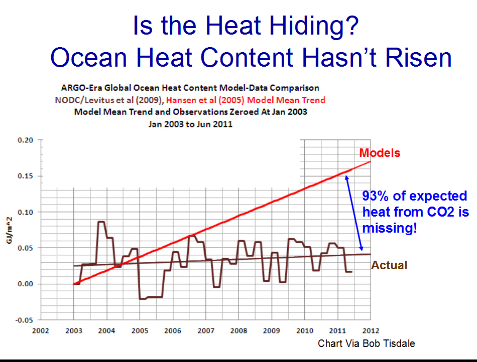
harmlessly off to space or taken up into the ocean, which appears to have warmed
during the ARGO decade at a rate equivalent to just 0.05 K decade–1 – well within the
very large measurement and coverage uncertainties (each ARGO buoy has to try to
monitor 200,000 km3 of ocean). [Note to Christopher Monckton: the atmosphere and
greenhouse gases cannot "generate heat"]
Since the atmosphere has not warmed during the ARGO decade, it is not illegitimate
to deduce that at least the upper or mixed stratum has not warmed during the past
decade, for if it had done so the atmosphere – three orders of magnitude less dense
than the ocean, and intimately mixed with it at its interface by tropical afternoon
convection in low latitudes and baroclinic eddies in the extratropics – ought to have
warmed too.
I have raised the Bode problem several times in my lectures on climate, with
interesting results. At a lecture to an audience including several IPCC lead authors in
Tasmania some years back, I showed the Bode plot and a lead author who had been
sneering all the way through the lecture suddenly sat bolt upright, peered at the
screen and said, “Have you published this?” No, I said, I was still working on it. “But
you must,” he cried out. “This changes everything.” Yes, I said, it does.
Reactions were rather more mixed at a meeting of the climate monitoring panel of
the World Federation of Scientists two years ago. A mathematician said, “Well,
perhaps the output is just undefined at a loop gain exceeding 1” (except that in an
electronic circuit the output is defined by the Bode equation: the voltage reverses
itself as the loop gain crosses the singularity). A climatologist growled, “Well, it
works perfectly well up to a loop gain of 0.8” (which, a little too conveniently, is the
IPCC’s implicit upper bound).
The most startling result was three years ago, before a learned society, when I
debated the climate with a professor who, until then, had been a Thermageddonite.
But he took one look at the plot of the Bode equation, went white, realized at once
that it could not possibly apply to the climate, and wrote to me resolving to do
further work on it. He has now concluded, like me and for similar reasons, that
climate sensitivity to a CO2 doubling will be around 1 K, and may well be less.
Whether he will be able to get a leading climate journal to publish so heretical a
result, of course, is quite another matter in these days of science as politics.
The significance of Bode is this. If it does not apply to climate, that is the end of high
sensitivity; and that, in turn, is the end of the climate scare. That is why, pace Dr
Istvan, we thought it right to include a mention of the Bode problem in our paper.Dr Istvan
says we have made a mistake in assuming that all loop gains greater than
approximately 0.1 would imply an unstable climate when, as noted above, the climate
has been near-perfectly thermostatic for the best part of a million years. With
respect, he perpetrates the same error as the climatologist at the World Federation of
Scientists. He assumes that there is an inflection point in the graph at 0.75 (which,
rounded up, is 0.8). However, the Bode function has no inflection point there, as I
know because I drew the plot point by point using a very precise architectural
drawing program.
Furthermore, Dr Istvan is missing two further steps in our argument that are vital to
understand. First, the reason why process engineers building electronic circuits
intended not to oscillate set an upper bound of 0.01 (or, in well-regulated conditions,
0.1) as an absolute maximum in the design specification is that the operating
conditions may not remain stable and the componentry may have been fabricated to
variable tolerances.
Mutatis mutandis, the climate, too, may suffer shocks – meteorites, supervolcano
explosions, Milankovic changes in the orbital characteristics, etc., etc. In feedback
amplification regime that looked anything like the Bode plot, IPCC’s implicit central
estimate of 0.65 for the feedback sum is far too close to the singularity. There would
have been several points in the past 810,000 years where a feedback sum that large
would have driven the feedback-sum beyond unity, leading to violent results that are
simply absent from the record.
Secondly, if one must use Bode at all then one must do as the process engineers do,
and accept that at the singularity Bode is impossible in all circumstances, for the
equation predicts an infinite output response to a finite input. Even in circuitry,
where at least the current is reversible at the singularity and the voltage is a bare
output that plays no part in equilibrating the circuit after a perturbation, selfevidently
asymptotic upper and lower bounds constraining the output voltage exist.
Indeed, if one hooks up an oscilloscope to a circuit and serially drives the feedback
above unity and then lets it relax back below unity, a sine-wave will result. The
positive and negative splines of the singularity are not merely truncated: the curve at
all points either side of the singularity is tempered.
What are the values of the asymptotes in the climate object? Given the sandwiching
of the atmosphere between two vast heat-sinks, and given the consequent
thermostasis that is indeed inferred in the ice-core temperature reconstructions,
there is no particular reason to suppose that the asymptotes will be markedly further
apart today than the 6-7 K interval in the ice-core record. And we are already only 2.5
K below the upper-bound asymptote.
Dr Istvan also challenges the complexity of our derivation of the closed-loop gain:
however, he has not noticed the series of simple equations we provide throughout the
paper – some of them for the first time. Our derivations were sometimes step-by-step
because our paper was in part pedagogical: we were, for the first time, letting the
daylight in on the magic, and that meant explaining some concepts for the novice in a
certain amount of necessary detail.
Dr Istvan also says that our discussion of the Bode equation is irrelevant to our
equation and its evaluation. Not so: it is vital, because in the IPCC’s
(mis)understanding two-thirds of all global warming is generated by the use of that
equation. That is where the big error lies in the models. That is the chief reason why
they over-predict global warming.
Curiously, a climate modeller at NASA GISS made a similar mistake to Dr Istvan,
even going so far as to say the Bode equation was not used in the climate models at
all. I referred him to not one but two papers by James Hansen, the creator of the
GISS model, each of which discussed the applicability of the Bode equation. One
paper even derived it from first principles not inelegantly – but without taking into
account the constraints on its applicability that I have set forth here.
Dr Istvan is kind enough to say that “the mathematical derivation of the irreducibly
simple equation is impeccable”. Several Thermageddonite commentators, in their
habitually sour fashion, have put it this way: “It’s not new.” But it is new to most of
those who will download our paper.
Dr Istvan says that the transience fraction (i.e., the fraction of equilibrium warming
that will occur a given number of years after an instantaneous forcing) might be more
simply derived than in our paper. However, we were not concerned only with
deriving today’s value from IPCC’s values for other parameters in the study of climate
sensitivity: we wanted to empower researchers to trace their own path from
instantaneous forcing via transient response to equilibrium response, even allowing
for such arcana as the possibility of a response lag owing to the “missing heat” hiding
in the deep ocean (though the ocean notion has zero empirical evidence to support
it).
Indeed, one of our reviewers told us he thought that the “missing heat” pretext for
the complex models’ failure was now well established in the literature. So we
searched the literature and found four papers pushing the ocean notion – let us call
them Smith et al., Wesson et al., Aguirre et al. and Aranzabal et al.
On closer inspection, the four were members of the same group of authors. Each had
taken it in turn to be lead author, exploiting the fact that papers are usually cited
simply as “Smith et al.”, rather than as “Smith, Wesson, Aguirre y Aranzabal”. And
their notion had been spankingly debunked by a group at the Chinese Academy of
Sciences. We also found some two dozen mutually incompatible excuses for the failure of
models to predict the Great Pause. The ocean notion was just one of these. Either
way, to the startlement of the reviewer, our model – with a tunable array variable to
allow the user to choose his own pathway from instantaneity to equilibrium – was,
though simple, sophisticated enough to represent (if desired) response lags such as
that conjured into being by the proponents of the ocean notion.
Dr Istvan was good enough to put our model through its paces. He went through the
principal temperature feedbacks that we had mentioned in the paper, adjusted their
values as he thought right and found that the feedback sum was about 0.25, implying
a loop gain of 0.1 (i.e. the process engineers’ limit) and a system gain factor of 1.1,
giving a final climate sensitivity of 1.3 K (not quite sure how he got 1.75 K, starting
with a feedback sum of just 0.25 K W–1 m2).
Very kindly, Dr Istvan concludes that “The simple non-GCM models Trenberth
dismisses have great utility”. We agree. Indeed, our model turned up some very
interesting errors in the IPCC’s analysis, all of them calculated artificially to increase
climate sensitivity:
The assumption that “temperature feedbacks” would double or triple direct manmade greenhouse
warming is the largest error made by the complex climate models. Feedbacks may well reduce
warming, not amplify it.
The Bode system-gain equation models mutual amplification of feedbacks in electronic circuits,
but, when complex models erroneously apply it to the climate on the IPCC’s false assumption of
strongly net-amplifying feedbacks, it greatly over-predicts global warming. They are using the
wrong equation.
Modellers have failed to cut their central estimate of global warming in line with a new, lower
feedback estimate from the IPCC. They still predict 3.3 C° of warming per CO2 doubling, when
on this ground alone they should only be predicting 2.2 C° – about half from direct warming and
half from amplifying feedbacks.
Though the complex models say there is 0.6 C° manmade warming “in the pipeline” even if we
stop emitting greenhouse gases, the simple model – confirmed by almost two decades without any
significant global warming – shows there is no committed but unrealized manmade warming still
to come.
There is no scientific justification for the IPCC’s extreme RCP 8.5 global warming scenario that
predicts up to 12 Cº global warming as a result of our industrial emissions of greenhouse gases.
Have a look at the model for yourselves. Go to scibull.com (the unfortunately-chosen
website moniker for the newly-relaunched journal) and click on “Most Read
Articles”. We are no. 1 on the list, with 23,000 downloads of the abstract or the full
paper – an order of magnitude above our nearest rival in the journal’s 60-year
archive.We have some reason to suspect that the shrieking fury to which my co-author Willie
Soon was subjected once the usual suspects found they could not fault the paper
scientifically stems chiefly from our revelation that the Bode equation cannot be
applied to the climate without heavy modification. Those behind the climate scare
know this quite well. Now others know it too.


.PNG)
.PNG)