Showing posts sorted by relevance for query "arctic sea ice". Sort by date Show all posts

Sunday, August 10, 2014

Arctic sea ice could continue to recover for next 30+ years of negative AMO

The natural ~60-90 year Atlantic Multidecadal Oscillation [AMO] has been in its positive warming phase since 1976 and after ~30+ years of warming is "pausing" and transitioning to its ~30-45 year negative phase [cooling]:


Coincidentally, satellite observations of Arctic sea ice began in 1979 at the start of the positive warming phase of the AMO. The AMO transfers heat from the tropics to the Arctic and melts Arctic sea ice, thus the AMO and Arctic Sea Ice Index are inversely related:


Five year moving average of the Arctic Sea Ice Index [red line] is inversely correlated to the Atlantic Multidecadal Oscillation [AMO] five year moving average shown in green. 
The AMO index "paused" right around the same time global temperatures "paused," perhaps related to solar control of climate and ocean oscillations. 


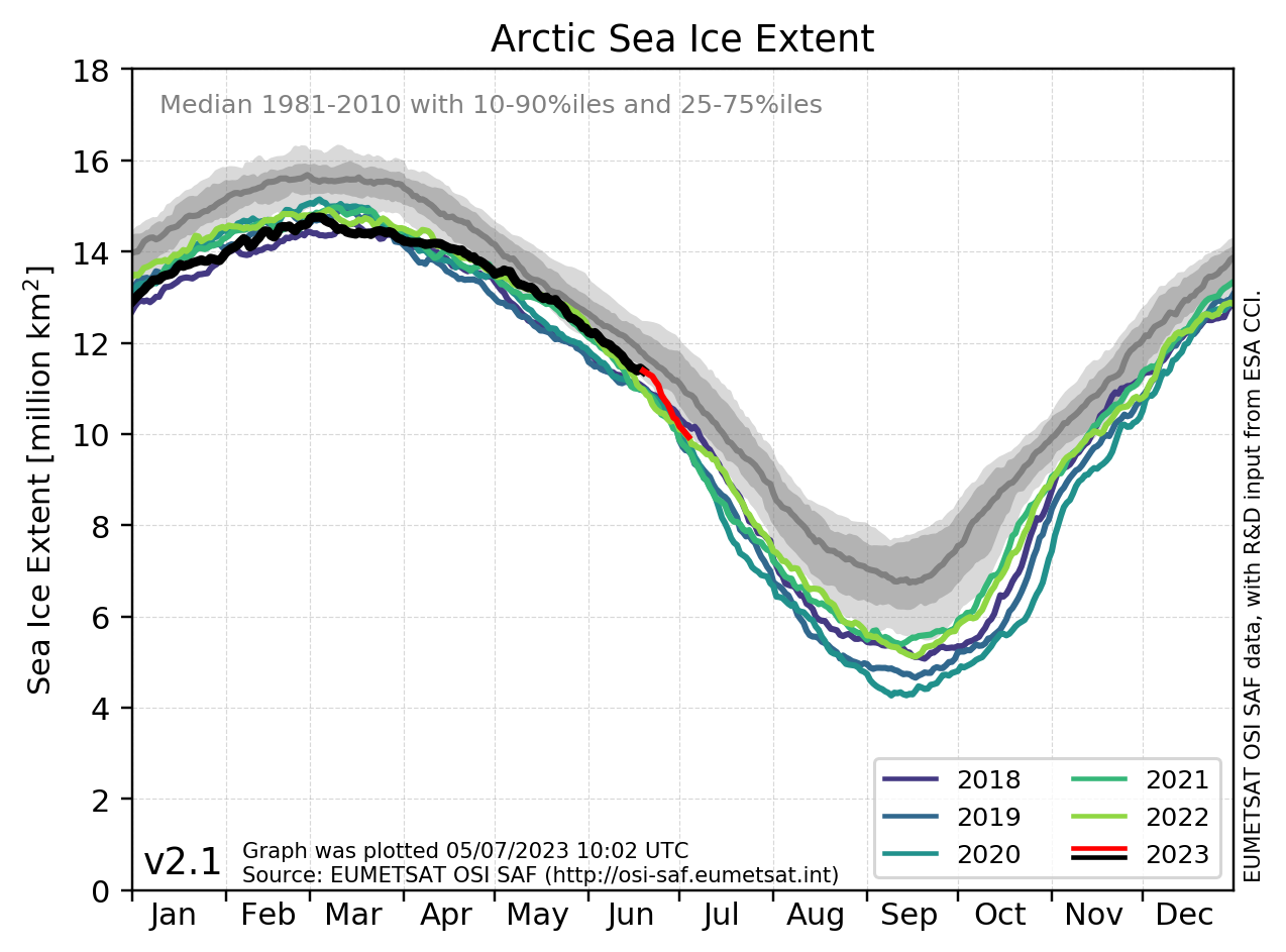
Perhaps this is why Arctic sea ice is having a dramatic recovery this year and is within one standard deviation of the mean:


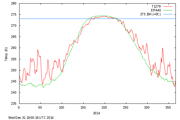
Might this explain why Arctic temperatures have been below the mean every single day during this summer's melt season?:


Thanks to the Arctic sea ice recovery and record high levels of Antarctic sea ice, global sea ice is now back to levels seen 35 years ago


The AMO may now be entering a new ~30-45 year negative phase. If this nutty denier theory is correct, Arctic sea ice could continue to recover for the next 30+ years of the negative phase of the AMO, even if you hang on to your dirty carbon-pollution-spewing SUV. 

Climate experts claim Arctic sea ice and just about everything else in climate is governed by a man-made CO2 "control knob" and most definitely not related to natural ocean oscillations such as the AMO (which in turn are controlled by solar activity), ocean warming from accumulated solar energy, and storm activity. 

Repost:

New paper finds Arctic sea ice is controlled by natural cycles
A paper published today in Geophysical Research Letters finds Arctic sea ice extent is determined primarily by the natural ~60-90 year cycle of the Atlantic Multidecadal Oscillation [AMO], not greenhouse gases.

According to the authors, "Arctic sea ice is intrinsically linked to Atlantic multidecadal [natural] variability" finding a ~60-90 year cycle of "Covariability between sea ice and Atlantic multidecadal variability as represented by the Atlantic Multidecadal Oscillation (AMO) index is evident during the instrumental record."

The paper adds to many other peer-reviewed publications finding changes in Arctic sea ice are primarily related to natural variability of ocean and atmospheric oscillations, storm and wind activity, and not changes in greenhouse gases.

A Signal of Persistent Atlantic Multidecadal Variability in Arctic Sea Ice

Martin W. Miles et al


Satellite data suggest an Arctic sea ice–climate system in rapid transformation, yet its long-term natural modes of variability are poorly known. Here, we integrate and synthesize a set of multi-century historical records of Atlantic Arctic sea ice, supplemented with high-resolution paleo proxy records, each reflecting primarily winter/spring sea ice conditions. We establish a signal of pervasive and persistent multidecadal (~60–90 year) fluctuations that is most pronounced in the Greenland Sea, and weakens further away. Covariability between sea ice and Atlantic multidecadal variability as represented by the Atlantic Multidecadal Oscillation (AMO) index is evident during the instrumental record, including an abrupt change at the onset of the early 20th century warming (ETCW). Similar covariability through previous centuries is evident from comparison of the longest historical sea ice records and paleo proxy reconstructions of sea ice and the AMO. This observational evidence supports recent modelling studies that have suggested that Arctic sea ice is intrinsically linked to Atlantic multidecadal [natural] variability. This may have implications for understanding the recent negative trend in Arctic winter sea ice extent, although because the losses have been greater in summer, other processes and feedbacks are also important.


The AMO, PDO, and NAO have all been linked to solar activity as the driver [possible lunar tidal influence as well].

Tuesday, September 16, 2014

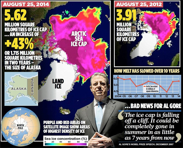
Preliminary Arctic sea ice summer minimum up 48% since 2012 minimum

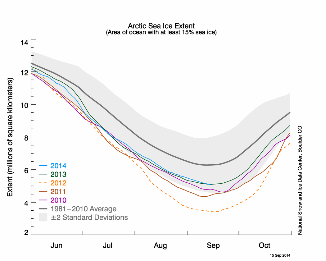
According to a report from the NSIDC released today, Arctic sea ice extent at the end of the summer melt season stood at 5.07 million square kilometers as of yesterday, although "weather conditions near the ice edge heavily influence the timing of the minimum, which has occurred as late as September 23. We are now a day past the 1981 to 2010 average minimum date of September 15."

Compared to the Arctic sea ice minimum of 3.41 million square kilometers on September 16, 2012, sea ice extent was ~48% higher at 5.07 million km2 on September 15, 2014. 


The NSIDC also confirms the Northwest Passage remains closed at the end of the melt season, despite Al Gore's claim "the entire North 'polarized' cap will disappear" by 2013. 


Regardless, much of the intense fixation on Arctic sea ice extent is likely misplaced due to dominant influences of natural variation over AGW on Arctic sea ice extent.


Melt season ending

September 16, 2014  NSIDC

The end of this year’s Arctic sea ice melt season is imminent and the minimum extent will be slightly lower than last year’s, making it the sixth lowest extent in the satellite record. Earlier in the month, a small area of the Laptev Sea ice edge was within five degrees of the North Pole. This appears to be the result of persistent southerly winds from central Siberia. Meanwhile, Antarctic sea ice is poised to set a record maximum this year, now at 19.7 million square kilometers (7.6 million square miles) and continuing to increase.


Overview of Conditions


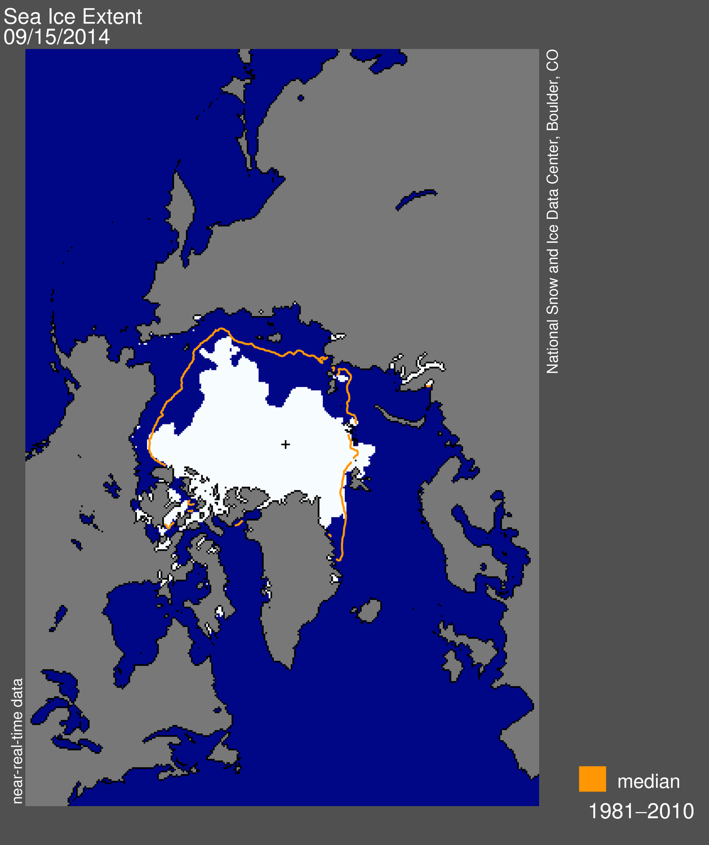
Figure 1. Arctic sea ice extent for September 15, 2014 was 5.07 million square kilometers (1.96 million square miles). The orange line shows the 1981 to 2010 average extent for that day. The black cross indicates the geographic North Pole. Sea Ice Index data. About the data  Credit: National Snow and Ice Data Center High-resolution image

Arctic sea ice extent for September 15 was 5.07 million square kilometers (1.96 million square miles). This is only 30,000 square kilometers (11,600 square miles) below the same date last year, yet sea ice extent remains low compared to the long-term 1981 to 2010 average. As is typical for this time of year, weather conditions near the ice edge heavily influence the timing of the minimum, which has occurred as late as September 23. We are now a day past the 1981 to 2010 average minimum date of September 15.

Conditions in context


Figure 2. The graph above shows Arctic sea ice extent as of September 15, 2014, along with daily ice extent data for four previous years. 2014 is shown in blue, 2013 in green, 2012 in orange, 2011 in brown, and 2010 in purple. The 1981 to 2010 average is in dark gray. Sea Ice Index data. Credit: National Snow and Ice Data Center High-resolution image

Sea ice extent declined at a rate of 28,700 square kilometers (11,100 square miles) per day through the first half of September. This is nearly twice as high as the 1981 to 2010 average rate of decline for this period of 16,200 square kilometers (6,200 square miles) per day. As was the case for the beginning of the month, extent remains below average in all sectors of the Arctic except for a region in the Barents Sea, east of Svalbard. There are areas of fairly low concentration ice north of the East Siberian and Chukchi seas that may still melt out or compact from wind-driven drifting.

However, as in 2013, a large area in the East Siberian Sea remains ice covered, helping to keep the overall extent higher for this time of year than observed since 2007. Last summer that area was covered by first-year ice that did not melt out under cooler-than-average conditions. This year, a region of second-year ice appears to have helped stabilize ice loss there.

The Northwest Passage remains closed, while the Northern Sea Route is still largely clear of ice.

A new ice edge


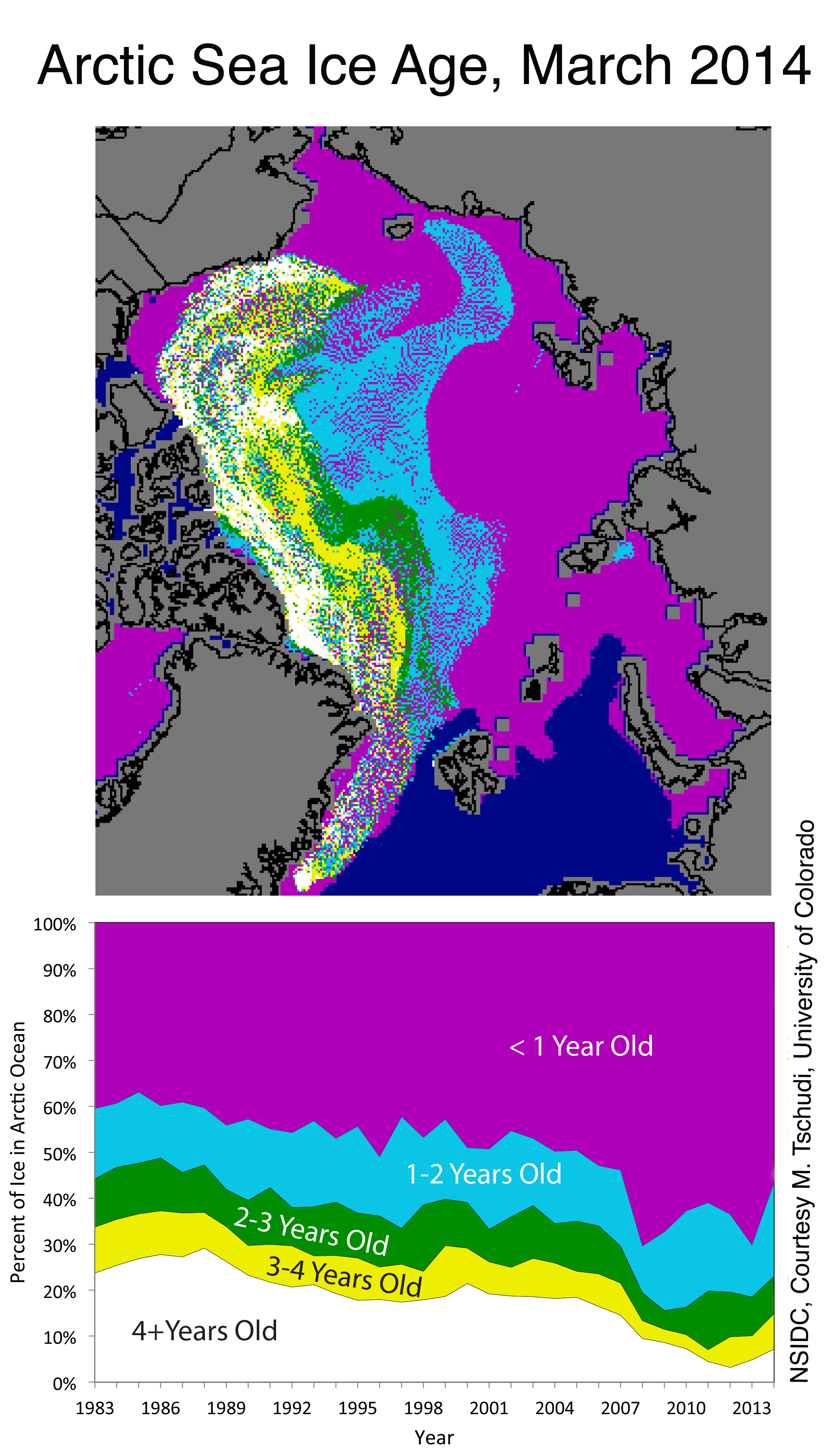
Figure 3a. The map at top shows the ages of ice in the Arctic at the beginning of March 2014; the bottom graph shows how the percentage of ice in each age group has changed from 1983 to 2014 . Credit: NSIDC, courtesy M. Tschudi, University of Colorado High-resolution image

Through the first half of September, the ice edge slowly retreated north of the Laptev Sea and is now within five degrees latitude of the North Pole. This is the most northerly position that the ice edge has been recorded over the period of satellite observations in this region. A large part of this region was also ice free in 2007. The reasons for the strong ice retreat in this sector are, at present, not entirely clear but we offer some initial insights.


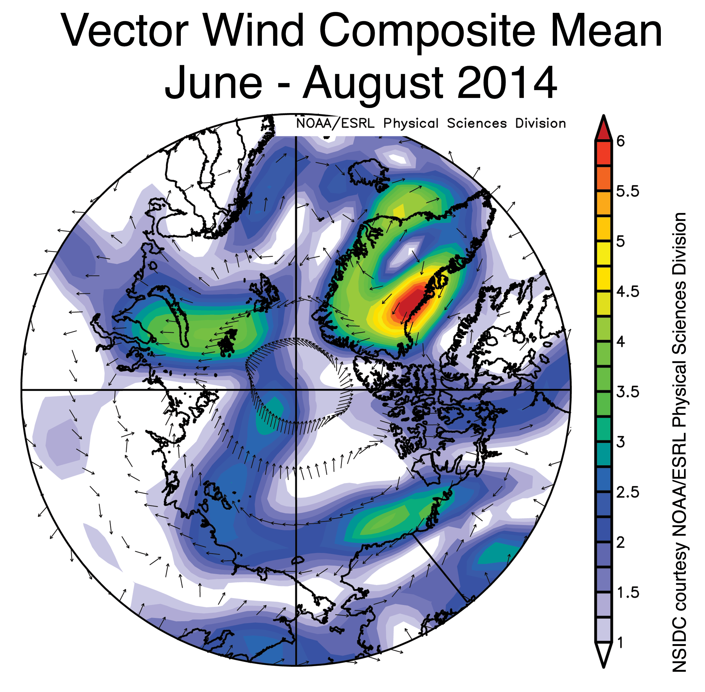
Figure 3b. This map shows surface wind patterns over the Arctic region from June to August 2014. Credit: NSIDC courtesy NOAA/ESRL Physical Sciences Division High-resolution image

In April, we discussed the pattern of ice age across the Arctic as the melt season began. In general, younger ice tends to be thinner ice. Areas of young ice are more likely to melt out during the summer than areas of old ice. The ice age figure from that post, reproduced here (Figure 3a), shows a strong northward extension of ice less than one year of age along the same general longitudes that open water has developed. Given the general circulation of the sea ice away from the Siberian shores, this area of thin ice prone to melting out would have tended to advance further northward through the melt season. Indeed, average sea level pressures this summer featured a pattern of surface winds particularly conducive to transporting thinner ice northward in the Laptev Sea sector (Figure 3b). To the east, winds were calmer and an arm of older, thicker second-year ice there may have helped to limit melt out and northward advection.

Sea surface temperature update


Figure 4. These maps show Arctic sea surface temperatures (left) and temperature anomalies (right) for August 2014, in degrees Celsius. Sea surface temperature data are from the National Climatic Data Center’s OIv2 “Reynolds” data set, a blend of satellite (Advanced Very High Resolution Radiometer) and in situ data designed to provide a bulk or mixed layer temperature. Ice edge data are from NSIDC near-real time passive microwave data. Credit: Mike Steele/University of Washington High-resolution image

As one may expect with an early retreat of sea ice, sea surface temperatures in the Laptev Sea were higher than average by up to 5 degrees Celsius (9 degrees Fahrenheit), with up to 3 degrees Celsius (5 degrees Fahrenheit) anomalies extending north of 80 degrees North for the first time since 2007. Early ice retreat and high sea surface temperatures are not unusual for this area and have appeared every summer since 2007, with the exception of 2008. The date of ice opening in the Laptev Sea is not particularly unusual in 2014 either. Open water and warming ocean temperatures started in early June. However, this summer there was a rapid northward progression of the ice edge in this area, especially along about longitude 140 degrees East, which allowed the sun to warm the resulting open water.

Over other parts of the Arctic, sea surface temperatures were not particularly noteworthy, except for cooler-than-average conditions in the northern Barents and Kara seas where the ice has remained extensive compared to recent summers. This reverses a recent trend toward warming and ice retreat in these areas, noted in last year’s sea surface temperature update. Preliminary analysis indicates that these changes are forced by local meteorological conditions, rather than oceanic heat transport by Atlantic water.
Further reading

Steele, M., S. Dickinson, and J. Zhang. 2014. Seasonal ice loss in the Beaufort Sea: Toward synchronicity and prediction. Journal of Geophysical Research-Oceans. In review.

Monday, February 24, 2014

Why "The Arctic is melting!" is just Mann-made global warming scaremongering

Reblogged from Real Science:

Understanding The 1979 Arctic Ice Cherry Pick

Posted on February 22, 2014 by stevengoddard

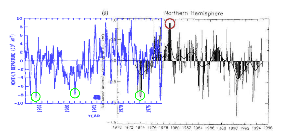
Climate fraudsters like to claim that Earth began in 1979, the year of peak Arctic sea ice. The graph below shows why. If they started their graph in 1954, there would be almost no downwards trend to the present.


journals.ametsoc.org/doi/pdf/10.1175/1520-0485(1979)009<0580>2.0.CO%3B2


Reblogged from Global Warming Solved:

Is the Arctic melting?

Ice trends

The satellite records only began in October 1978, however. This coincided with the start of a recent warming trend in the Arctic. Before that, from the 1950s-1970s, Arctic temperatures were cooling. So, it is quite likely that in the decades immediately before the satellite records began, average Arctic sea ice extent was actually increasing, but we just weren’t monitoring it. It seems that the Arctic sea ice extent naturally goes through periods of expansion, followed by periods of contraction.


In case you’re unsure about which is which, the Arctic is the polar region in the north (the one with polar bears, etc.) and the Antarctic is the polar region in the south (the one with penguins, etc.)

In this essay, we look at what we know about Arctic sea ice extent.

1. The satellite era
2. What do we know about Arctic temperatures?
3. The pre-satellite era
4. The great Arctic explorers
5. Conclusions

1. The satellite era

Every winter, the sea ice in the polar regions grows, but then in the summer, it melts again.


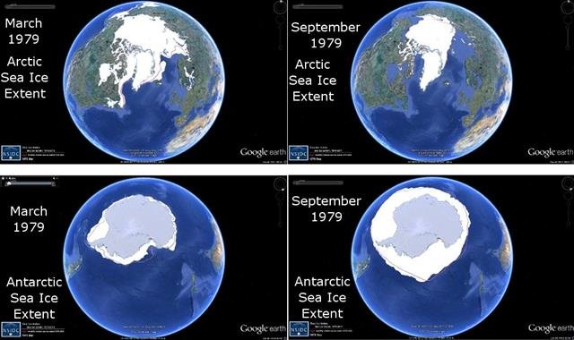
Figure 1. Minimum and maximum sea ice extents for northern and southern hemispheres in 1979. Click to enlarge.Since winter and summer are reversed between the southern and northern hemispheres, this means that as the Arctic sea ice reaches its maximum extent in March, the Antarctic sea ice is reaching its minimum extent. By September, the situation has reversed (minimum Arctic and maximum Antarctic sea ice). This can be seen from the Google Earth images in Figure 1 (generated using data from NSIDC).


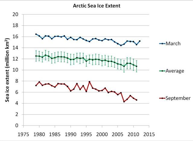
Figure 2. Trends in maximum (March), minimum (September) and average annual sea ice extents for the Arctic, since records began in 1979. Error bars for the average value correspond to the standard errors. Click to enlarge.This cyclical pattern occurs every year. However, since satellite records began in 1979, the maximum (March) and minimum (September) sea ice extents in the Arctic seem to have been gradually decreasing. This can be seen from Figure 2 (generated using NSIDC data).


This has led many people to worry that it is man-made global warming which is causing the Arctic sea ice to melt, and that humans are therefore destroying an entire ecosystem, threatening animals such as polar bears.

As a result, much of the research in the Arctic in recent years has become dominated by a heavy focus on man-made global warming, rather than studying the Arctic as a fascinating region in itself.


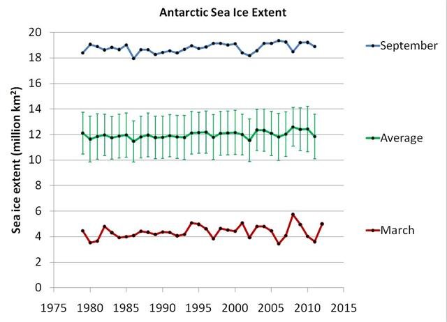
Figure 3. Trends in maximum (September), minimum (March) and average annual sea ice extents for the Antarctic, since records began in 1979. Error bars for the average value correspond to the standard errors. Click to enlarge.Interestingly, even though you might expect “global” warming to occur globally, in the southern half of the world, the Antarctic sea ice extent doesn’t seem to have changed much (see Figure 3). This apparent paradox has puzzled those who believe the Arctic melting is due to man-made global warming.

As a result, some groups have struggled to come up with explanations as to why man-made global warming is not causing melting of Antarctic sea ice. For example, Zhang, 2007 (Open access) proposed that warmer waters off Antarctica might make the water less salty, and that maybe this would stop the ice from melting. We believe a much simpler explanation is that the changes in the Arctic sea ice arenot due to the “man-made global warming” assumed by current climate models. If the explanation is not “CO2-related”, then we would no longer need to worry about why the models don’t match the data – it would just mean that the models are wrong.

At any rate, since the Antarctic sea ice extent doesn’t seem to be declining, the public concern over sea ice seems to be confined to the Arctic. With that in mind, let us limit our discussion in this essay to the Arctic, i.e., the region which has shown a decrease in polar sea ice. The fact that the Arctic sea ice seems to have been steadily decreasing “since records began” does initially seem alarming. However, as we will see below, this is because “the records” only began in October 1978, as the satellites weren’t launched until then.
There may be some problems with the satellite estimates of sea ice extent, e.g., see here. Estimating sea ice extent from satellites is a complex problem – the satellites aren’t actually photographing the amount of ice, so it’s not a simple case of looking at a photograph and saying “oh, there’s some ice there, and none there”.

Instead, they measure microwave emissions. Analysts then try to convert those measurements into estimates of sea ice. These conversions rely on several different assumptions being valid. If there are problems with those assumptions, it may affect the reliability of the satellite estimates.

However, for the purposes of this post, we assume that the satellite estimates are reliable.

2. What do we know about Arctic temperatures?


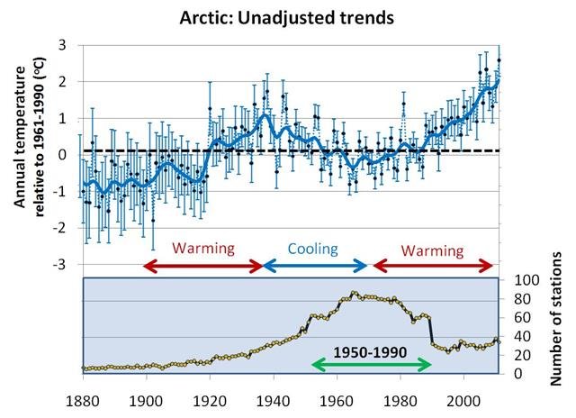
Figure 4. Top panel: Unadjusted average temperature trends of all GHCN stations in the Arctic Circle. Thick solid line corresponds to a smoothed average (11 point binomial). Bottom panel: Number of stations available in a given year. Taken from our Urbanization bias III paper. Click to enlarge.In Figure 4, the average annual temperature trends for the Arctic are shown (the graph is taken from our “Urbanization bias III” paper – Provide link!). We can see that there has indeed been a warming trend since the late 1970s. However, if we look at the rest of the data, the problem of the sea ice record only beginning in 1979 should become obvious – the warming trend since the 1970s followed acooling trend from the 1940s. If the sea ice records had started just a bit earlier, they would probably have first shown sea ice growth!

Before the 1940s-1970s Arctic cooling, there also seems to have been another warming period (1900s-1930s). We do not have enough weather records to reliably tell what happened to Arctic temperatures before the 20th century, but it is at least plausible that similar cooling and warming periods also occurred then. It seems that temperatures in the Arctic naturally alternate between periods of warming and periods of cooling.

In the next sections, we will argue that sea ice conditions in the late 1970s were relatively severe. So, the fact that the Arctic sea ice extent seems to have been decreasing since then is not an indicator of “unusual and dramatic melting of the Arctic”. Instead, it seems that the satellite monitoring of the Arctic sea ice just coincidentally started at the wrong time, i.e., just when the last Arctic cooling period had ended!

But before we get to that, some readers might say, “If you look at the graph of Arctic temperatures since 1880, the linear trend shows warming, so that must be due to human activity!”. Well, no.

First, the trends are non-linear, so the “linear trend” is irrelevant. There are periods of both warming and cooling, so the linear trend changes depending on where you start and end your analysis. If you want to, you can technically calculate a “linear trend” for any (x,y) dataset, but if it is non-linear data, as is the case here, then it is a meaningless calculation. See our “Urbanization bias I” paper for more discussion (Provide link!).

Second, there is no reason to assume warming must be “man-made”, rather than just a natural occurrence. For instance, Prof. Syun-Ichi Akasofu, the founding director of the International Arctic Research Center (retired in 2007) argues that the world may still be recovering naturally from the Little Ice Age of the 18th and 19th centuries. Dr. Willie Soon has found that the warming and cooling trends in the Arctic are actually strongly correlated to changes in solar activity, e.g., Soon, 2009 (Abstract; Google Scholar access).


Figure 5. Locations of stations used for constructing the above graph. The 6 stations with data for at least 75 of the last 80 years are shown with white squares. Click to enlarge.Finally, as we discuss in our “Urbanization bias III” paper (Provide link!), there are very few stations with long records available for the Arctic (see the bottom panel of the earlier figure showing Arctic temperature trends). The map in Figure 5 shows the locations of all the available stations – only six of the stations have data for 75 of the last 80 years, and five of them are from a relatively small region (northern Scandinavia).

This means that if there are non-climatic biases in any of the station records, it could strongly alter the apparent trends of the average “Arctic temperatures”. This is a particular concern for periods when the number of stations were very low, e.g., there appears to have been a sudden warming step change at about 1920, but there were only a few stations actually available then, so it is hard to know if the apparent step change was genuinely climatic.

For example, many of the Arctic stations are airport stations, and improvements in the airport infrastructure, such as insulation of permafrost-based runways (e.g., Instanes & Mjureke, 2005) could easily have introduced warming biases in recent decades.

Also, you might not think urbanization bias would be a major problem in the Arctic, since most of the big cities are at lower latitudes. But, in tundra conditions, even modest urbanization can introduce significant biases.


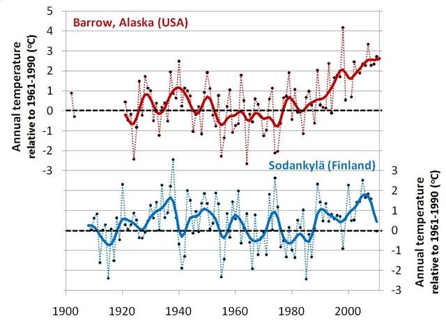
Figure 6. Comparison of temperature trends for two of the six Arctic stations with relatively long and complete records. Thick solid lines correspond to smoothed averages (11 point binomial). Taken from our Urbanization bias III paper. Click to enlarge.For instance, even though Barrow, Alaska (USA) still has a relatively small population (4,500 in 2000), urbanisation has led to a considerable urban heat island there in recent years – see Hinkel et al., 2003(Open access). This would have introduced an artificial warming trend which would make the recent warm period seem warmer than it actually was. In comparison, the rural Sodankylä, Finland station also shows a warming trend since the late 1970s, but it followed a cooling period from the 1940s, and its warmest year was actually in 1937 (see Figure 6).

So, unfortunately, the data is really too limited to make definite conclusions (e.g., only six stations with data for 75 of the last 80 years, and at least one of them is known to have an urban heat island). It may well be that the recent warm period was warmer than the early 20th century warm period, as the raw data suggests… Or it may be that biases in the raw data are substantial, and the early 20th century warm period was just as warm as the recent warm period, or maybe even warmer.

Whatever the case, it is clear that the Arctic seems to alternate between periods of warming and periods of cooling. Hence, the fact that “the Arctic sea ice has been decreasing since records began” is merely down to the fact that the records only began in 1978. In the next sections, we will try to estimate how sea ice varied, before the satellite era.

3. The pre-satellite era

A few groups have attempted to construct sea ice estimates for the pre-satellite era using various combinations of land, ship, submarine, buoy and aircraft measurements made over the years, e.g., the Chapman & Walsh dataset or the Zakharov dataset (Note that the server for the Zakharov dataset is not always online, so the link sometimes doesn’t work). These datasets represent a considerable amount of compilation work, and probably could be used to extract useful climate information. But, as we will discuss below, there are too many inconsistencies in the data sources for a simple analysis.

Some people have used these datasets to argue that the decreasing trend during the satellite era is an acceleration of an already decreasing trend in the pre-satellite era. For instance on the “Open Mind” blog, the blogger “Tamino” has used the Walsh & Chapman dataset to claim that the satellite era melt is unprecedented, e.g., here. However, these datasets should not be used for estimating long term trends. The problem is that such datasets are actually composite datasets constructed by compiling together as many measurements as the researchers can for a given year.

The measurement sources vary dramatically over the years. For instance, in Siberia, measurements up until the late 1930s were mostly from shipping lane reports, while after the late 1930s they mostly came from aircraft measurements. In addition, the actual regions with available data varied substantially over the decades. So, a sea ice estimate for a region constructed from shipping reports in the 1920s might not be directly comparable to an estimate for the same region from the 1940s made from aircraft measurements. Hence, they cannot be used for calculating long term trends.

We suspect that with careful work and calibration, it might be possible to construct useful long term trends for at least part of the pre-satellite era. However, they don’t seem to be reliable yet. For example, we saw in the previous section, that the temperature records show a period of substantial warming followed by a period of substantial cooling up to the satellite era. But, pre-satellite sea ice datasets such as Walsh & Chapman’s don’t show any of that variability in the pre-satellite era.

So, unfortunately, we can’t use the pre-satellite estimates for assessing how unusual the recent melting has (or hasn’t) been. Fortunately, there are ways of assessing how unusual the sea ice in 1979 (at the start of the satellite era) was. If the claim that the recent Arctic melting is unusual and due to man-made global warming were true, then this would mean that the sea ice extent in September 1979 was relatively low (September being the month of minimum sea ice in the Arctic).

In the following section, we will assess this claim, by trying to answer the question, “Would the great 19th and early 20th Arctic explorers have been able to carry out all their voyages if they had attempted it during 1979 conditions?” If September 1979 sea ice extent was already quite low, then 1979 conditions would have been relatively easy for them. However, as we will see, many of the early explorers managed to get much further than they could have in 1979. In other words, at the time of those voyages, the sea ice extent was probably much lower than it was at the start of the satellite era.

Sunday, March 23, 2014

New paper finds Arctic sea ice was much less than present-day during the Holocene Climate Optimum ~6,000 years ago

A new paper published in Quaternary Science Reviews finds Arctic sea ice extent and thickness was much less than present-day conditions during the Holocene Climate Optimum from ~10,000-6,000 years ago. According to the authors, "Arctic Ocean sea ice proxies generally suggest a reduction in sea ice during parts of the early and middle Holocene (∼6000–10,000 years Before the Present) compared to present day conditions." 

The authors show 8 different proxy studies reveal extended periods lasting hundreds of years without perennial sea ice in the Arctic [ice-free conditions], and find solar insolation explains these changes. 
Top graph shows simulated annual mean sea ice thickness [orange curve] was much less during the Holocene Climate Optimum ~13,000-6,000 years ago compared to the end of the 20th century at right side of graph. Bottom graph shows multiple proxies of sea ice with darker green indicating periods of less sea ice. Modern sea ice is at high levels in comparison to the rest of the Holocene. 
Fig. 4. 
Annual mean sea ice thickness for the three different simulations (Panel a) compared with results from published paleo-sea ice studies (Panel b). Black curve: constant surface albedo; red curve: dynamic surface albedo parameterization. The simulation implemented with a dynamic surface albedo parameterization was run from present time and backwards to address the importance of the initial state of the sea ice cover. The annual mean sea ice thickness from this simulation (orange curve) reveals a hysteresis of ∼1000 years. The annual mean insolation at 80°N shown with a stippled curve is based on the algorithm presented by Berger (1978). To compare the results from different paleo-sea ice studies a scale of sea ice concentration was inferred using the approach by Jakobsson et al. (2010). This scale must be considered as highly qualitative because none of the paleo-sea ice proxies provide absolute measures of past sea ice concentrations. 

Arctic Ocean perennial sea ice breakdown during the Early Holocene Insolation Maximum 

Abstract

Arctic Ocean sea ice proxies generally suggest a reduction in sea ice during parts of the early and middle Holocene (∼6000–10,000 years Before the Present) compared to present day conditions. This sea ice minimum has been attributed to the northern hemisphere Early Holocene Insolation Maximum (EHIM) associated with Earth's orbital cycles. Here we investigate the transient effect of insolation variations during the final part of the last glaciation and the Holocene by means of continuous climate simulations with the coupled atmosphere–sea ice–ocean column model CCAM. We show that the increased insolation during EHIM has the potential to push the Arctic Ocean sea ice cover into a regime dominated by seasonal ice, i.e. ice free summers. The strong sea ice thickness response is caused by the positive sea ice albedo feedback. Studies of the GRIP ice cores and high latitude North Atlantic sediment cores show that the Bølling–Allerød period (c. 12,700–14,700 years BP) was a climatically unstable period in the northern high latitudes and we speculate that this instability may be linked to dual stability modes of the Arctic sea ice cover characterized by e.g. transitions between periods with and without perennial sea ice cover.

Wednesday, August 3, 2011

New paper finds Arctic sea ice strongly linked to varying storm activity

Warmists often claim changes in Arctic sea ice are a consequence of allegedly-anthropogenic global warming. However, a paper published today in the Journal of Geophysical Research finds that "dramatic interannual changes" in Arctic sea ice extent are due to varying storm activity in the months of May-July, which impacts "cloud cover and ice motion, and consequently sea ice melt." The authors find fewer cyclones in the Arctic Ocean "appear to favor a low sea ice area at the end of the melt season." Thus, the alleged connection between AGW and Arctic sea ice extent becomes all the more elusive.
JOURNAL OF GEOPHYSICAL RESEARCH, VOL. 116, D15105, 10 PP., 2011

Dramatic interannual changes of perennial Arctic sea ice linked to abnormal summer storm activity 

Key Points:

Interannual changes of Arctic sea ice are related to varying storm activity
Fewer summer storms favor low sea ice at the end of the melt season
Storms impact the cloud cover and ice motion, and consequently sea ice melt

James A. Screen et al

The perennial (September) Arctic sea ice cover exhibits large interannual variability, with changes of over a million square kilometers from one year to the next. Here we explore the role of changes in Arctic cyclone activity, and related factors, in driving these pronounced year-to-year changes in perennial sea ice cover. Strong relationships are revealed between the September sea ice changes and the number of cyclones in the preceding late spring and early summer. In particular, fewer cyclones over the central Arctic Ocean during the months of May, June, and July appear to favor a low sea ice area at the end of the melt season. Years with large losses of sea ice are characterized by abnormal cyclone distributions and tracks: they lack the normal maximum in cyclone activity over the central Arctic Ocean, and cyclones that track from Eurasia into the central Arctic are largely absent. Fewer storms are associated with above-average mean sea level pressure, strengthened anticyclonic winds, an intensification of the transpolar drift stream, and reduced cloud cover, all of which favor ice melt. It is also shown that a strengthening of the central Arctic cyclone maximum helps preserve the ice cover, although the association is weaker than that between low cyclone activity and reduced sea ice. The results suggest that changes in cyclone occurrence during late spring and early summer have preconditioning effects on the sea ice cover and exert a strong influence on the amount of sea ice that survives the melt season.

Thursday, October 25, 2012

New study finds growth of Antarctic sea ice accelerated 53% since 2006


Opposite Behaviors? Arctic Sea Ice Shrinks, Antarctic Grows


September 2012 witnessed two opposite records concerning sea ice. Two weeks after the Arctic Ocean's ice cap experienced an all-time summertime low for the satellite era (left), Antarctic sea ice reached a record winter maximum extent (right). But sea ice in the Arctic has melted at a much faster rate than it has expanded in the Southern Ocean, as can be seen in this image by comparing the 2012 sea ice levels with the yellow outline, which in the Arctic image represents average sea ice minimum extent from 1979 through 2010 and in the Antarctic image shows the median sea ice extent in September from 1979 to 2000. (Credit: NASA/Goddard Space Flight Center Scientific Visualization Studio and NASA Earth Observatory/ Jesse Allen)
ScienceDaily (Oct. 23, 2012) — The steady and dramatic decline in the sea ice cover of the Arctic Ocean over the last three decades has become a focus of media and public attention. At the opposite end of Earth, however, something more complex is happening.

A new NASA study shows that from 1978 to 2010 the total extent of sea ice surrounding Antarctica in the Southern Ocean grew by roughly 6,600 square miles every year, an area larger than the state of Connecticut. And previous research by the same authors indicates that this rate of increase has recently accelerated, up from an average rate of almost 4,300 square miles per year from 1978 to 2006. [an increase of 53% between 1978-2010 vs. 1978-2006 rate]

"There's been an overall increase in the sea ice cover in the Antarctic, which is the opposite of what is happening in the Arctic," said lead author Claire Parkinson, a climate scientist with NASA's Goddard Space Flight Center, Greenbelt, Md. "However, this growth rate is not nearly as large as the decrease in the Arctic."

Earth's poles have very different geographies. The Arctic Ocean is surrounded by North America, Greenland and Eurasia. These large landmasses trap most of the sea ice, which builds up and retreats with each yearly freeze-and-melt cycle. But a large fraction of the older, thicker Arctic sea ice has disappeared over the last three decades. The shrinking summer ice cover has exposed dark ocean water that absorbs sunlight and warms up, leading to more ice loss.

On the opposite side of the planet, Antarctica is a continent circled by open waters that let sea ice expand during the winter but also offer less shelter during the melt season. Most of the Southern Ocean's frozen cover grows and retreats every year, leading to little perennial sea ice in Antarctica.

Using passive-microwave data from NASA's Nimbus 7 satellite and several Department of Defense meteorological satellites, Parkinson and colleague Don Cavalieri showed that sea ice changes were not uniform around Antarctica. Most of the growth from 1978 to 2010 occurred in the Ross Sea, which gained a little under 5,300 square miles of sea ice per year, with more modest increases in the Weddell Sea and Indian Ocean. At the same time, the region of the Bellingshausen and Amundsen Seas lost an average of about 3,200 square miles of ice every year.

Parkinson and Cavalieri said that the mixed pattern of ice growth and ice loss around the Southern Ocean could be due to changes in atmospheric circulation. Recent research points at the depleted ozone layer over Antarctica as a possible culprit. Ozone absorbs solar energy, so a lower concentration of this molecule can lead to a cooling of the stratosphere (the layer between six and 30 miles above Earth's surface) over Antarctica. At the same time, the temperate latitudes have been warming, and the differential in temperatures has strengthened the circumpolar winds flowing over the Ross Ice Shelf.

"Winds off the Ross Ice Shelf are getting stronger and stronger, and that causes the sea ice to be pushed off the coast, which generates areas of open water, polynyas," said Josefino Comiso, a senior scientist at NASA Goddard. "The larger the coastal polynya, the more ice it produces, because in polynyas the water is in direct contact with the very cold winter atmosphere and rapidly freezes." As the wind keeps blowing, the ice expands further to the north.

This year's winter Antarctic sea ice maximum extent, reached two weeks after the Arctic Ocean's ice cap experienced an all-time summertime low, was a record high for the satellite era of 7.49 million square miles, about 193,000 square miles more than its average maximum extent for the last three decades.

The Antarctic minimum extents, which are reached in the midst of the Antarctic summer, in February, have also slightly increased to 1.33 million square miles in 2012, or around 251,000 square miles more than the average minimum extent since 1979.

The numbers for the southernmost ocean, however, pale in comparison with the rates at which the Arctic has been losing sea ice -- the extent of the ice cover of the Arctic Ocean in September 2012 was 1.32 million square miles below the average September extent from 1979 to 2000. The lost ice area is euivalent to roughly two Alaskas.

Parkinson said that the fact that some areas of the Southern Ocean are cooling and producing more sea ice does not disprove a warming climate.

"Climate does not change uniformly: The Earth is very large and the expectation definitely would be that there would be different changes in different regions of the world," Parkinson said. "That's true even if overall the system is warming." Another recent NASA study showed that Antarctic sea ice slightly thinned from 2003 to 2008, but increases in the extent of the ice balanced the loss in thickness and led to an overall volume gain.
The new research, which used laser altimetry data from the Ice, Cloud, and land Elevation Satellite (ICESat), was the first to estimate sea ice thickness for the entire Southern Ocean from space.

Records of Antarctic sea ice thickness are much patchier than those of the Arctic, due to the logistical challenges of taking regular measurements in the fierce and frigid waters around Antarctica. The field data collection is mostly limited to research icebreakers that generally only travel there during spring and summer -- so the sole means to get large-scale thickness measurements is from space.

"We have a good handle of the extent of the Antarctic sea ice, but the thickness has been the missing piece to monitor the sea ice mass balance," said Thorsten Markus, one of the authors of the study and Project Scientist for ICESat-2, a satellite mission designed to replace the now defunct ICESat. ICESat-2 is scheduled to launch in 2016. "The extent can be greater, but if the sea ice gets thinner, the volume could stay the same."

Sunday, September 14, 2014

New paper links Arctic sea ice extent to absorption of sunlight by clouds

A new paper published in the Journal of Geophysical Research Atmospheres finds Arctic sea ice concentrations at the low of each summer are related to absorption of sunlight by cloud cover at the top of the atmosphere in early summer, a phenomenon "not represented in most of current climate models."

According to the authors, 
"absorbed solar radiation at the top of the atmosphere in early summer (May–July) plays a precursory role in determining the Arctic sea ice concentration in late summer (August–October)"   
"this intimate delayed...relationship is not represented in most of current climate models. Rather, the models tend to over-emphasize internal sea ice processes in summer."
Alarmists focus on Arctic sea ice as the supposed canary in the coal mine for CAGW, but many papers have demonstrated natural variability is more likely responsible for the trends in Arctic sea ice than man-made CO2, including the natural Atlantic Multidecadal Oscillation, Atlantic Meridional Overturning Circulation [AMOC], wind  & storm activity, and long-term solar variability. This new paper suggests another way that natural variability controls Arctic sea ice extent via cloud cover, another possible solar amplification mechanism  via the cosmic ray theory of climate.

Alarmists ignore the unspeakable all-time record highs in Antarctic sea ice extent broken over each of the past three years, as do climate models, which laughably predicted the opposite of a decrease in Antarctic sea ice extent more so than Arctic sea ice. 

Alarmists also claim current Arctic sea ice changes are "unprecedented" while ignoring proxy data indicating Arctic sea ice was much less than present-day during the Holocene Climate Optimum ~6,000 years ago, Arctic temperatures were warmer than the present multiple times over past 1357 years, the Medieval Warming Period in the Arctic was warmer than the present, Alaskan glaciers are about the same size as during the Medieval Warm Period, etc., etc.


Connecting early summer cloud-controlled sunlight and late summer sea ice in the Arctic


Yong-Sang Choi, Baek-Min Kim, Sun-Kyong Hur, Seong-Joong Kim, Joo-Hong Kim, Chang-Hoi Ho

This study demonstrates that absorbed solar radiation (ASR) at the top of the atmosphere in early summer (May–July) plays a precursory role in determining the Arctic sea ice concentration (SIC) in late summer (August–October). The monthly ASR anomalies are obtained over the Arctic Ocean (65°N–90°N) from the Clouds and the Earth's Radiant Energy System during 2000–2013. The ASR 
[absorbed solar radiation] changes primarily with cloud variation. We found that the ASR [absorbed solar radiation] anomaly in early summer is significantly correlated with the SIC [Arctic sea ice concentration] anomaly in late summer (correlation coefficient, r ≈ −0.8 with a lag of 1 to 4 months). The region exhibiting high (low) ASR anomalies and low (high) SIC anomalies varies yearly. The possible reason is that the solar heat input to ice is most effectively affected by the cloud shielding effect under the maximum TOA solar radiation in June and amplified by the ice-albedo feedback. This intimate delayed ASR-SIC relationship is not represented in most of current climate models. Rather, the models tend to over-emphasize internal sea ice processes in summer.

Wednesday, September 22, 2010

Paper: Current Arctic Sea Ice is More Extensive than Most of the past 9000 Years

A peer-reviewed paper published in the Canadian Journal of Earth Sciences finds that western Arctic sea ice extent at the end of the 20th century was more extensive than most of the past 9000 years. The paper also finds that the western Arctic sea ice extent was on a declining trend over the past 9000 years, but recovered beginning sometime over the past 1000 years and has been relatively stable and extensive since. The paper also demonstrates that even though western annual sea ice extent has been less than the present throughout most of the last 9000 years, low sea ice has consistently failed to cause a planetary albedo 'tipping point' claimed by warmists.

Although it seems like a day doesn't go by without an alarmist headline or blog posting obsessing over the daily Arctic sea ice statistics (and never about Antarctic sea ice extent which reached a record high this year), this paleo-climate perspective takes all the wind out of alarmist sails. Satellite assessment of sea ice conditions is only available beginning in 1979 (around the time the global cooling scare ended), with only sparse data available prior to 1979. The alarmists at the NRDC fraudulently claim in a new video that due to "climate destruction," Arctic sea ice reached the lowest in history in 2010 (actually the low since 1979 was in 2007 and 2010 was the 3rd or 4th lowest depending on the source). Probably wouldn't bring in many donations if they mentioned the truth: the 21st century has some of the highest annual western Arctic sea ice extents over the past 9000 years.

The figure below comes from the paper, but has been modified with the red notations and rotated clockwise. The number of months the sea ice extent is greater than 50% is shown on the y axis. Time is on the x axis starting over 9000 years ago up to the present. Warming periods are shown in gray with the Roman and Medieval warming periods (RWP/MWP) notated, the Minoan Warming Period about 5000 years ago, and another older unnamed warming period. The last dot on the graph is the end of the 20th century and represents one of the highest annual sea ice extents.
Holocene fluctuations in Arctic sea-ice cover: dinocyst-based reconstructions for the eastern Chukchi Sea Canadian Journal of Earth Sciences, 45: 1377-1397

Authors: J.L. McKay, A. de Vernal, C. Hillaire-Marcel, C. Not, L. Polyak, and D. Darby

Abstract: Cores from site HLY0501-05 on the Alaskan margin in the eastern Chukchi Sea were analyzed for their geochemical (organic carbon, d13Corg, Corg/N, and CaCO3) and palynological (dinocyst, pollen, and spores) content to document oceanographic changes during the Holocene. The chronology of the cores was established from 210Pb dating of near- surface sediments and 14C dating of bivalve shells. The sediments span the last 9000 years, possibly more, but with a gap between the base of the trigger core and top of the piston core. Sedimentation rates are very high (*156 cm/ka), allowing analyses with a decadal to centennial resolution. The data suggest a shift from a dominantly terrigenous to marine input from the early to late Holocene. Dinocyst assemblages are characterized by relatively high concentrations (600–7200 cysts/cm3) and high species diversity, allowing the use of the modern analogue technique for the reconstruction of sea-ice cover, summer temperature, and salinity. Results indicate a decrease in sea-ice cover and a corresponding, albeit much smaller, increase in summer sea-surface temperature over the past 9000 years. Superimposed on these long-term trends are millennial-scale fluctuations characterized by periods of low sea-ice and high sea-surface temperature and salinity that appear quasi-cyclic with a frequency of about one every 2500–3000 years. The results of this study clearly show that sea-ice cover in the western Arctic Ocean has varied throughout the Holocene. More importantly, there have been times when sea-ice cover was less extensive than at the end of the 20th century.
Arctic summer sea surface temperatures are also currently lower than much of the past 9000 years
note this is version 2.0 of this post updated to repeatedly emphasize this drilling site was located in the western Arctic. see comments below for details.

Thursday, April 17, 2014

New paper finds current abrupt changes in Arctic are typical of the past 66 million years

An important review paper published today in Quaternary Science Reviews demonstrates that the rapid changes in the Arctic which have been blamed on man by alarmists are in fact within the norm of frequent, large and abrupt changes for the entire Cenozoic Era [past 66 million years].

According to the paper, "Globally, the general trend of increasing air surface temperature over the last 15 years has slowed in recent years, and is currently four times less than predicted by simulations [of the latest IPCC climate models] (Fyfe et al., 2013). However, over the same interval, global atmospheric CO2 level has continued to increase (Francey et al., 2013) and the Arctic Ocean has experienced a rapid decline in summer sea ice extent and thickness (Stroeve et al., 2012) (Fig. 1). The lack of a strong correlation between global average air temperature, atmospheric CO2 and Arctic summer sea ice provides one example that shows that Arctic environmental changes are heavily influenced by complex interplays between different feedback mechanisms." i.e. not the simplistic explanation by warmists that all changes in the Arctic are man-made.

According to the authors, "Instead of interpreting changes almost exclusively as near linear responses to external forcing (e.g. orbitally-forced climate change [or man-made greenhouse gases]), research is now concentrated on the importance of strong feedback mechanisms that in our palaeo-archives often border on chaotic behaviour. The last decade of research has revealed the importance of on-off switching of ice streams, strong feedbacks between sea level and ice sheets, spatial and temporal changes in ice shelves and perennial sea ice, as well as alterations in ice sheet dynamics caused by shifting centres of mass in multi-dome ice sheets."

The paper states, "Perhaps the next paradigm shift is towards recognising the unstable nature of Arctic cryosphere and Arctic environmental change more widely? That instability likely makes predicting the future a real challenge."

The dynamic Arctic
Research campaigns over the last decade have yielded a growing stream of data that highlight the dynamic nature of Arctic cryosphere and climate change over a range of time scales. As a consequence, rather than seeing the Arctic as a near static environment in which large scale changes occur slowly, we now view the Arctic as a system that is typified by frequent, large and abrupt changes. The traditional focus on end members in the system – glacial versus interglacial periods – has been replaced by a new interest in understanding the patterns and causes of such dynamic change. Instead of interpreting changes almost exclusively as near linear responses to external forcing (e.g. orbitally-forced climate change [or man-made greenhouse gases]), research is now concentrated on the importance of strong feedback mechanisms that in our palaeo-archives often border on chaotic behaviour. The last decade of research has revealed the importance of on-off switching of ice streams, strong feedbacks between sea level and ice sheets, spatial and temporal changes in ice shelves and perennial sea ice, as well as alterations in ice sheet dynamics caused by shifting centres of mass in multi-dome ice sheets. Recent advances in dating techniques and modelling have improved our understanding of leads and lags that exist in different Arctic systems, on their interactions and the driving mechanisms of change. Future Arctic research challenges include further emphases on rapid transitions and untangling the feedback mechanisms as well as the time scales they operate on.

1. Introduction

The Arctic has a prominent role in scientific debate on global change. This is a consequence from that the region is changing faster than almost anywhere on Earth and from that such dynamic change in the Arctic has been a characteristic of the entire Cenozoic Era. Thus, quantitative palaeoclimate reconstructions suggest that Arctic temperature changes have been three or four times the corresponding hemispheric or globally averaged changes over the past 4 Ma (Miller et al., 2010).
Globally, the general trend of increasing air surface temperature over the last 15 years has slowed in recent years, and is currently four times less than predicted by simulations within Phase 5 of the Coupled Model Intercomparison Project (CMIP5) (Fyfe et al., 2013). However, over the same interval, global atmospheric CO2 level has continued to increase (Francey et al., 2013) and the Arctic Ocean has experienced a rapid decline in summer sea ice extent and thickness (Stroeve et al., 2012) (Fig. 1). The lack of a strong correlation between global average air temperature, atmospheric CO2 and Arctic summer sea ice provides one example that shows that Arctic environmental changes are heavily influenced by complex interplays between different feedback mechanisms. These include changes in glacier/ice sheet extent, snow cover and sea ice distribution that affect surface albedo, and atmospheric and oceanic circulation patterns. The Arctic also influences environmental change at lower latitudes, primarily through the global thermohaline circulation and modulation of atmospheric CO2 and CH4 concentrations (Overpeck et al., 1997).
Full-size image (245 K)
Fig. 1. 
The dynamic Arctic illustrated on different time scales. Orbital forcing (g) constitutes the main overarching climate driver on millennial time scales. Considering this parameter alone, the present interglacial is likely to last at least another 50,000 years (Berger and Loutre, 2002), although the net effect from feedbacks is far from known and remains a research challenge. On millennial time scales the sea level record follows from a build-up and decay of large ice sheets (f) with large feedback effects from, for example, changes of land/ocean distribution. The sea ice (a–e) is perhaps the Arctic component that best illustrates how the dynamics of the climate system is operating on different time scales.
Environmental variability in the Arctic is increasingly viewed as the norm, and there is a growing recognition that today's Arctic cryosphere (glaciers, sea ice, permafrost, gas hydrates) and biosphere (terrestrial, lacustrine, and marine) are not in steady state; they have changed and will continue to change in response to climate and other perturbations. Recognition that the Arctic has likely never been in steady state is a challenge to those of interested in reconstructing past change. What, for example, is the purpose of seeking to define a reconstruction of the maximum extent of an entire ice sheet, such as at the Last Glacial Maximum (LGM), if the age of that maximum extent was diachronous and the ice sheet was not in equilibrium with its climate?
The Arctic Palaeoclimate and Its Extremes (APEX) program was initiated in October 2004 in Brorfelde, Denmark, with the aim of better understanding the magnitude and frequency of past Arctic climate variability, especially the “extremes” versus the “normal” conditions of the climate system. The goal has been to highlight Arctic palaeoclimate changes through an interdisciplinary approach that integrates marine and terrestrial science, and through using modelling that is constrained by boundary conditions set by field observations.
It is the nature of the subject that research completed under APEX, as under its predecessors PONAM (Polar North Atlantic Margin: Late Cenozoic Evolution) (Elverhøi et al., 1998) and QUEEN (Quaternary Environments of the Eurasian North) (Thiede et al., 2004), has gravitated towards understanding end-member records of extreme events rather than signatures of transitions, be they gradual or abrupt, or indeed dynamic change within a particular state. Indeed, notwithstanding the attraction of such end-members, including our growing ability to apply reliable tools to identify maximum and minimum situations (e.g. maximum extent of ice, climate optimum, episodes of high relative or global sea level) in both time and space, we are increasingly appreciative of the fact that Arctic cryospheric and oceanic changes are time-transgressive.
From the perspective of Earth's orbit around the Sun, the present interglacial is expected to last for an exceptionally long interval, perhaps more than another 50,000 years (Berger and Loutre, 2002) (Fig. 1). The implication is that CO2 forcing and dynamic feedback mechanisms will dictate climate change long into the future, and for this reason the forcing and feedbacks that link these processes are important future targets for Arctic research in the years to come.
This special issue contains a suite of articles that mark the completion of the APEX program. Collectively they provide a state-of-the-art record of current knowledge regarding Arctic Quaternary environmental change, and here we aim to review progress achieved under the PONAM-QUEEN-APEX programs and highlight the main scientific challenges that they have left us with.

2. History and current status

2.1. Palaeoglaciology

The year 1875 was a break-through year for Agassiz' (1840) Ice Age Theory, with the work of Croll (1875) on multiple ice ages through time marking the birth of palaeoglaciology as a scientific subject. Palaeoglaciology aims to outline the history of former ice sheets and cast light on their dynamics through time (Andersen and Borns, 1994), and over the past 120 years there have been ever more sophisticated reconstructions that seek to define the former extents of the Eurasian ice sheets e.g., Andersen, 1981, Hughes et al., 1981 and Svendsen et al., 2004; see also reviews in Fastook and Hughes (2013) and Ingólfsson and Landvik (2013).
It is interesting to ask the question “How far have we advanced our understanding of palaeoglaciology sinceGeikie (1894) published his maps of ice sheet extents over Europe, the British Isles and Scandinavia?” A partial answer to this question can be found by comparing these original maps with current versions, as we do in Fig. 2. What is astounding from this exercise is how remarkably similar Geikie's map from 1894 is to, by example, the recent reconstructions by QUEEN (Fig. 2). Such a comparison begs the question as to whether this means that the discipline has been treading water for much of the last century? We argue that it does not; that there are good reasons why the general maximum extents on base maps are little changed and there have indeed been major advances in our understanding of former ice sheet extents and in their dynamics. However, we also argue that we must now make a greater effort to illustrate the dynamics of these glacial system on maps and in other media; a far from trivial task!
Full-size image (138 K)
Fig. 2. 
Ice sheet extent published on the “Glacial Map of Asia” by Geikie (1894) compared with the Last Glacial Maximum (LGM) and Saalian ice sheet margins by the QUEEN program (Svendsen et al., 2004).
As pointed out by Ingólfsson and Landvik (2013), there is a fundamental problem with regional palaeoglacial reconstructions because they synthesise large amounts of field data that contain problems, notably different spatial resolutions and often problematic age controls. The outcome of such efforts is therefore commonly a compromise of best fit reconstructions that simplify or over-look time-transgressive changes and ignore ice sheet dynamics; the ice sheets are reconstructed as if they are always close to steady-state equilibrium. In Europe and Eurasia, the resulting reconstructions tend to depict the ice sheets as relatively stable, concentric or single-domed rather than unstable and multi-domed, and, although ice streams may be acknowledged, the dynamic linking of the ice sheets to global and regional sea levels is often not accounted for. These reconstructions do not allow for the understanding that marine-based ice streams are inherently unstable (Jamieson et al., 2012) nor do they fully recognise that different sectors of an ice sheet experienced different histories, depending on the topography/bathymetry, sub-glacial conditions and glacial dynamics, as well as climate and sea-level forcing. These problems are particularly evident for the marine sectors of former ice sheets, because ice shelves and floating ice tongues are highly dynamic, yet do not leave clearly identifiable imprints of their maximum extents (Jakobsson et al., 2014). Landvik et al. (2014) also note that the distribution of glacigenic bedforms, which are used as the main data source for reconstructing past ice flows, are most informative about the most recent events with older landforms susceptible to erosion. There is, therefore, considerable work to be done to reconcile glacial geomorphology data with the dynamic ice margin behaviour predicted by ice sheet models (Kirchner et al., 2011). This includes reconciling the resolution of ice sheet models with the temporal and spatial complexities of the glacial geomorphological evidence that documents ice sheet build-up and decay (Evans et al., 2009).
A growing appreciation of the dynamic nature of Arctic glacier and ice sheet change also challenges the traditional view of the link between palaeoglaciology and climate change, across glacial–interglacial and stadial–interstadial transitions. Climatostratigraphic concepts are relatively easy to use at mid and low latitudes where glacial landforms and biostratigraphic indicators define end-members, but such concepts are much harder to use at higher latitudes (Backman et al., 2004 and Alexanderson et al., 2014). Consequently, ice sheet advances and retreats are all too often interpreted as evidence for climate events, disregarding the possibility that they may reflect changes in ice dynamics, e.g., rapid changes in grounding-line position in response to sea-level oscillations. For this reason, whilst some suggest that over past glacial–interglacial cycles, continental ice volume kept pace with slow, multi millennial-scale changes in climate forcing (Rohling et al., 2013b), there is an increasingly recognition that system feedbacks (Fig. 1) can readily cause ice sheet collapse, independent of strong climate forcing (Hughes, 2011, Ã“ Cofaigh, 2012, Mangerud et al., 2013 and O'Leary et al., 2013). Understanding causal links that lead to such “tipping point” behaviour is a major challenge of Arctic palaeoglaciology.
There are several important advances in our understanding of Quaternary ice sheet extents and behaviour that extend beyond the one dimensional representation of an isochronous ice limit drawn on a map. First, the development of new dating methods, notable cosmogenic exposure dating, combined with improved understanding of the basal thermal regime of ice sheets, has enabled reconstructions of the former temporal dimension of the vertical extent of former ice sheets (Alexanderson et al., 2014 and Stroeven et al., 2014). This has challenged long-standing paradigms that interpreted trim lines as evidence for the upper limits of ice sheets and instead has led to a more nuanced appreciation of the importance of cold-based ice, and the recognition that former ice thicknesses were greater than previously thought. This knowledge has important implications for reconstructions of down-ice flow lines, as well as overall ice volume at glacial maxima.
A second advance is the appreciation of the important role of ice streams and their geometry in controlling the dynamic behaviour of large parts of an ice sheet (e.g. Andreassen et al., 2014, Batchelor and Dowdeswell, 2014 and Kleman and Applegate, 2014). Recent observations and reconstructions show that large-scale reorganizations of ice streams can significantly affect ice sheet dynamics over relatively short time scales (Winsborrow et al., 2012). In Greenland today, we see three or four major ice streams dominating the dynamic mass loss from the ice sheet, and that these ice streams can accelerate or slow-down in an unpredictable manner (Joughin et al., 2011). By thinning and accelerating, West Antarctic ice streams are contributing about 10% of the observed global sea level rise, and much of this ice loss is from Pine Island Glacier alone (Dutrieux et al., 2013). Such is the importance of ice streams to our understanding of the overall dynamics of the former ice sheets, during ice build-up and decay, that considerable effort is directed at unravelling their sensitivity to different forcing.
Conventional theory suggests that ice sheets and ice streams that are grounded below sea level are especially vulnerable to sea-level forcing, with the potential that sea-level jumps caused by ice sheet collapse can trigger further ice sheet instabilities. However, recent work is painting a more complex picture and challenging this long-held paradigm. For example, it has long been known that as an ice sheet loses mass, so the gravitational force of that ice mass on the adjacent ocean surface weakens (Simpson et al., 2009 and Woodroffe et al., 2014). This so-called “direct effect” causes relative sea level close to an ice sheet or ice stream that is losing mass to fall and, in theory, help stabilise the ice sheet margin by reducing water depths. In addition, removal of ice mass from a retreating ice sheet is often associated with glacio-isostatic rebound, a process that also causes relative sea level to fall. On the other hand, an example of a destabilizing effect is the sudden loss of an ice shelf that extends in front of an ice stream, that may result in rapid ice stream acceleration as the buttressing force the ice shelf exerted is lost (Rignot et al., 2004). We begin to map traces of abrupt ice stream break-ups and retreats from glacial landforms preserved in the seafloor of both the Antarctic (Jakobsson et al., 2011) and the Arctic (Andreassen et al., 2014 and Bjarnadóttir et al., 2014), that may well be the effects of former ice shelf collapses.
A third area of major advance is in our understanding of the dynamic effects of ocean forcing on ice sheet margin stability, especially those marine-based sections that are directly impacted by ocean temperatures. Warm water flowing beneath calving margins promotes significantly enhanced rates of basal melting, increased buoyancy and can lead to accelerated mass loss. This process is most clearly illustrated in the accelerated flow and retreat of Jakobshavns Isbrae (Greenland) in the last 15 years, during a period of time when warm Atlantic-sourced waters penetrated deep into the fjord system (Holland et al., 2008). A similar pattern of events is contributing the rapid collapse of Pine Island Glacier in Antarctica (Jacobs et al., 2011). This ocean coupling does not over-ride the importance of air temperature forcing, which remains a widely recognised control on ice sheet mass balance, including through the enhanced supply of meltwater to the base of ice sheets that may accelerate ice velocities. It does, though, exemplify the complex controls that combined to influence marine terminating ice sheets today.
A fourth advance is the significant progress made in reconstructing ice limits offshore, using remotely sensed imagery as well as sea bed sediment cores. Within the APEX project, we report important new understanding of the spatial extent of, for example, the Greenland Ice Sheet in West Greenland (Dowdeswell et al., 2014 and Lane et al., 2014). This is an essential development if we are to reconstruct how this ice sheet, and others that were grounded on the current continental shelf during initial deglaciation, responded to short-lived climate forcing such as the Younger Dryas (Ó Cofaigh et al., 2013).
In summary, the broad similarity between maps of Eurasian ice sheet extents drawn today and that of a hundred years ago or more masks significant advances in our understanding of the dynamic nature of ice sheet behaviour over a range of spatial and temporal scales. It is also true, however, that modern glaciological and oceanographic studies are not always appropriate analogues for the past, including previous interglacial (minima) ice-sheet configurations and during ice build-up and collapse. There is significant scope to improve our understanding of how ice sheets build during periods of high sea-level, whether the same atmosphere-ocean forcing that we see today operated in previous interglacials, or indeed whether the controls on ice sheet collapse during the exit from, for example, the LGM was typical of previous terminations or not.

2.2. Palaeoceanography

Reconstructions of oceanographic conditions in the central Arctic Ocean did not really begin until nearly half a century after Fridtjof Nansen compiled a bathymetric map that portrayed the central Arctic Ocean as a single deep featureless basin from a handful of lead line soundings acquired during the Fram Expedition1893–1896 ( Nansen, 1907). Extensive pack ice has prevented efficient mapping the Arctic Ocean seafloor, and each published map has systematically revealed a more complex seafloor, shaped by tectonics, ocean currents, and the glacial history, than the preceding one (e.g. Atlasov et al., 1964, Johnson et al., 1979, Perry et al., 1986 and Jakobsson et al., 2012). While the bathymetry provides a long-term paleoceanographic record of the interactions of bottom currents, ice, geochemical processes, and biological activity with the seafloor, sediment cores are required to decipher the palaeoceanography in detail.
Sediment core studies within the APEX program published in this special issue provide a range of new insights into the Arctic Ocean palaeoceanography (Chauhan et al., 2014, Gibb et al., 2014, Immonen et al., 2014, Löwemark et al., 2014 and Werner et al., 2014). These studies demonstrate how far we have progressed, specifically regarding the use of paleoceanographic proxies, since the first short cores raised from drifting ice islands in the 1950s and 1960s captured near surface sediments from the Arctic Ocean floor (Ericson et al., 1964 and Hunkins and Tiemann, 1977). Only the construction of research icebreakers in the 1980s allowed targeted expeditions to the Arctic to obtain long, large-volume sediment cores for palaeoceanographic reconstructions. During the QUEEN project, we learned that earlier ideas of extremely low sedimentation rates (Clark, 1970) were based on a misinterpretation of the palaeomagnetic pattern in the sedimentary record and that the rates were rather on the scale of centimetres per kiloyear than millimetres (Backman et al., 2004). While this finding substantially advanced our ability to use sediment cores to study palaeoceanography, the central Arctic Ocean sedimentation rate of centimetres per kiloyear is far from capturing the full dynamics and ongoing rate of change in the Arctic. It is also difficult to know what we capture with a proxy study of a sediment core; is what we reconstruct the extremes of paleoceanographic changes or a blurred averaged view? There is certainly not one answer to this questions, it will depend on several factors such as for example the proxy and core location.
The important role of the Arctic Ocean in driving the modern (interglacial) ocean circulation and heat transport was recognized by Nansen (1907), but due to the nearly land-locked Arctic Ocean physiographic configuration it was assigned a rather passive role during interglacials. It should be noted that Nansen's map from 1907 did not depict a deep Fram Strait simply because no soundings from the strait at that time had been collected. The CLIMAP reconstruction of the surface of the ice-age earth (CLIMAP Project Members, 1976) showed the Nordic Seas as perennially ice covered in the LGM and assumed that the Arctic Ocean had experienced the severest cold conditions. The last decades have seen a slow maceration of this contrasting view between glacial and interglacials. Evidence for a relatively strong advection of Atlantic Water to the Arctic in the LGM was found in the eastern Fram Strait where the associated moisture transfer from the sea surface to the atmosphere may have enhanced ice sheet growth on the Barents Sea (Hebbeln et al., 1994), and Hald et al. (2001) showed that Atlantic water repeatedly reached the polar North Atlantic during the Last Interglacial–Glacial cycle. It was assumed that this water mass reached only parts of the Eurasian Arctic (Sarnthein et al., 2003). This is in stark contrast to the interglacial Arctic Ocean, including present day conditions, when Atlantic Water contributes to the intermediate depth water masses well into the Makarov and Canada basins on the Amerasian side of the Arctic (Rudels et al., 2013).
Seafloor mapping, which began during the QUEEN program and continued during APEX, has revealed glacigenic landforms and ice grounded seabed in the central Arctic Ocean at depths >1000 m below present sea level, indicating the existence of marine based ice sheets including huge ice shelves (e.g. Polyak et al., 2001, Spielhagen et al., 2004, Niessen et al., 2013, Dove et al., 2014 and Jakobsson et al., 2014). How could these have existed if warm Atlantic Water entered the Arctic Ocean during glacials as well as interglacials? A conceptual model has been developed that now reconciles both the influx of Atlantic Water and the existence of deep drafting ice. This model suggests that the glacial palaeoceanography of the glacial Arctic was characterized by less fresh water influx resulting in a more diffuse and deeper halocline than today that forced the Atlantic Water deeper (Jakobsson et al., 2010). This model is supported by geochemical data from ostracods, as reported by Cronin et al. (2012). Their trace metal analyses of ostracod shells suggest that Atlantic Water penetrated basin-wide during the coldest phases of the Last Glacial, albeit at deeper depth than present. In addition, Hoffmann et al. (2013) showed that a persistent deep water exchange existed between the Arctic Ocean and North Atlantic during the last 35 ka. Apparently, the Arctic Ocean never lost the oceanographic connection to the rest of the World's ocean during the Last Glacial, and it thus contributed to the global ocean circulation over this time period.
Sea ice is one of the most dynamic components of the cryosphere as illustrated recently by the large yearly variation in the spatial extent of the Arctic Ocean summer sea ice (Comiso, 2011) (Fig. 1). The question most often asked is “When will there be sea ice free summers in the Arctic?” (Overland and Wang, 2013). The follow-up question is “Has the Arctic recently experienced sea ice free summers?” While the high frequency dynamic sea ice swings cannot be fully captured in sediment core studies, the general trends may be revealed from studies of various types of proxies for sea ice (Polyak et al., 2010 and de Vernal et al., 2013). Several studies suggest that the Early Holocene (∼6000–10,000 years BP) experienced less summer-sea ice than at present (e.g. Polyak et al., 2010, Funder et al., 2011 and Müller et al., 2012), although not all studies are showing the exact same pattern (Dyke and England, 2003). Stranne et al. (2014) show, using numerical modelling, that the sea ice during the Early Holocene potentially could have moved over to a seasonal regime with sea ice-free summers due to the insolation maxima the Earth experienced at that time (Fig. 1).

3. Discussions and future challenges

The history of Quaternary geology contains numerous examples of revolutions in our approaches to science that resulted from anomalies that could not be explained by the universally accepted paradigm. In glacial geology, Agassiz's (1840) Ice Age theory and Croll's (1875) and Milankovitch's (1920) astronomical theory mark paradigm shifts that fundamentally changed our views of how ice sheets and climate evolved over time (Hays et al., 1976). Our perception of how the large Quaternary ice sheets and the cryospheric system evolved over interglacial–glacial cycles has, however, changed slowly in recent decades. We find evidence from ice core and marine oxygen isotope data that the Late Pleistocene continental ice sheets were characterised by slow growth and rapid decay. Palaeoglaciological reconstructions typically reflect this pattern with continuous, isochronuous ice margins reconstructed by connecting geomorphological features, especially end moraines, to define events in ice expansion and retreat (Lüthgens and Böse, 2012). However, as we note above, the glacial landform record is strongly biased towards extreme events and terminations, whilst records of ice sheet dynamics during their growth phase are poorly preserved or not preserved at all.
As outlined above, the focus of Arctic palaeoglaciology has over the past few decades been on the LGM. The extents of LGM ice sheets are now reasonably well understood (Clark and Mix, 2002 and Clark et al., 2009) and we now know that growth of the ice sheets to their maximum positions occurred between 33.0 and 26.5 ka, and that nearly all ice sheets were at their LGM positions from 26.5 ka to 19–20 ka (Clark et al., 2009). We are now developing ever more sophisticated records of the dynamics of the deglaciations/terminations. Much of this new knowledge in the Arctic is drawn from newly collected marine geological data that reveals clear spatial and temporal variations in ice dynamics, with evidence for both active ice streaming and frozen-bed conditions at the maximum and during deglaciation (Ottesen and Dowdeswell, 2009, Winsborrow et al., 2010, Andreassen et al., 2014, Jakobsson et al., 2014 and Landvik et al., 2014). However, there is most likely much more information about the dynamics of the Arctic still to be extracted from palaeorecords as we improve our methods. In view of the advances in our understanding of the Arctic cryospheric system made during the International Polar Year (IPY) 2007–08 and the APEX program 2004–12, several challenges and research tasks stand out:
-
We need to focus on ice streams. The importance of ice streams for the geometry and stability of ice sheets has made the identification, location, and timing of ice stream activity essential for the reconstruction of palaeo-ice sheets and the interpretation of the associated landform record (Stokes and Clark, 2001, Bennett, 2003 and Batchelor and Dowdeswell, 2014);
-
We need to acknowledge in our reconstructions that the datasets that we work with tend to be strongly biased towards extreme events and terminations. This calls for a holistic approach where it is recognized that apparent mismatches and enigmatic data may be caused by the complexity and chaotic nature of the system rather than poor chronological or quality control of the data;
-
We need to focus on internal forcing and feedbacks in the Arctic system, particularly those that result in non-linear or chaotic behaviour such as changes in sea ice extent and ocean circulation;
-
We need to focus on rapid transitions and mode shifts, which in turn demands robust, high resolution chronologies;
-
We need to search for ultra-high resolution records (decadal to century-scale) that enable us to reconstruct past environmental change on time scales comparable to current and near-future environmental change;
-
We need to understand what were the leads and lags between different parts of the Arctic cryosphere/ocean, what caused them and how did they link to changes in the Southern Hemisphere?
-
We need to understand if Arctic ice sheets can grow quickly, during “warm” periods and if this can explain the high frequency sea-level variations seen in archives from low latitudes (Rohling et al., 2013a).
Perhaps the next paradigm shift is towards recognising the unstable nature of Arctic cryosphere and Arctic environmental change more widely? That instability likely makes predicting the future a real challenge.